State space models (SSM) are a tonne of fun. I sneaked one into a this post I did a while ago. In that post, I was recreating an analysis but using a state space model where the hidden state, the true $\beta$s were following a Gaussian Random Walk and what we observed was the growth in GDP. In this post, I’m going to explore a generalised version of the model - the linear-Gaussian SSM (LG-SSM).
The notation I am following is from Chapter 18 of Murphy’s Machine Learning book.
You can check out the (messy) notebook here.
What’s an LG-SSM
A state space model is like an HMM which I wrote about in these two blog posts. Instead of the hidden states being discrete, they are now continuous. So the model is:
\[\begin{aligned} \mathbf{z}_t &= g(\mathbf{u}_t, \mathbf{z}_{t-1}, \mathbf{\epsilon}_t)\\ \mathbf{y}_t &= h(\mathbf{z}_t, \mathbf{u}_t, \mathbf{\delta}_t) \end{aligned}\]$\mathbf{z_t}$ is our hidden state that is evolving as a function, $g$, of:
- the previous state, $\mathbf{z}_{t-1}$,
- the input, $\mathbf{u}_t$, and
- some noise $\mathbf{\epsilon}_t$.
What we observe is $\mathbf{y}_t$. This is a some function, $h$, of:
- the hidden state, $\mathbf{z}_t$,
- the input, $\mathbf{u}_t$, and
- some measurement error $\mathbf{\delta}_t$.
If we have a model where $g$ and $h$ are both linear functions and both of those error terms are Gaussian, we have linear-Gaussian SSM (LG-SSM). More explicitly, we have:
\[\begin{aligned} \mathbf{z}_t &= \mathbf{A}_t \mathbf{z}_{t-1} + \mathbf{B}_t \mathbf{u}_t + \epsilon_t\\ \mathbf{y}_t &= \mathbf{C}_t \mathbf{z}_t\,\,\,\, + \mathbf{D}_t \mathbf{u}_t + \delta_t \end{aligned}\]and the system and observation noises are Gaussian:
\[\begin{aligned} \epsilon_t &\sim \mathcal{N}(0, \mathbf{Q}_t)\\ \delta &\sim \mathcal{N}(0, \mathbf{R}_t) \end{aligned}\]In the growth regression model, $A_t$ was 1, $C_t$ was the GDP level, and $B_t$ & $D_t$ were 0.
Let’s simulate some data
size = 100
np.random.seed(15)

z0 = 0.5
ut = np.random.choice(np.arange(-2, 3), size=size)
zt = np.zeros(ut.shape[0])
yt = np.zeros(ut.shape[0])

A = 0.9
B = 2
C = 2
D = -1

Q = 2.9
R = 4
for i, u in enumerate(ut):
    if i == 0:
        zt[i] = z0
    else:
        zt[i] = A[i] * zt[i - 1] + B * ut[i] + np.random.normal(0, Q)
    yt[i] = C * zt[i] + D * (ut[i]) + np.random.normal(0, R)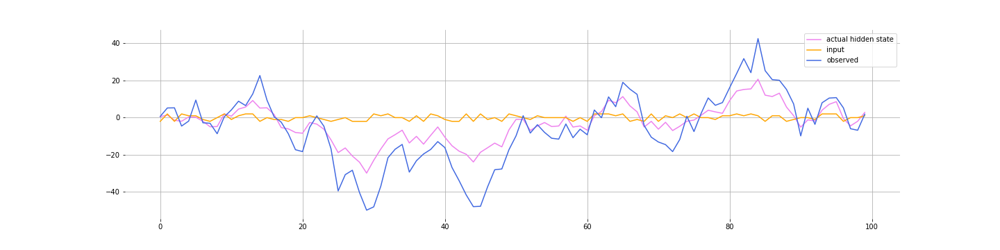
Note a few simplifications:
- We are just using scalars but $\mathbf{z}_t$ can be multi-dimensional and therefore $Q$, $A$ can be appropriately sized square matrices. A local linear trend model is an example.
- Similarly, so can $\mathbf{u}_t$
- Further, these parameters can be changing over time.
Kalman filtering / smoothing
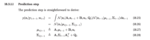
The nice thing about LG-SSM is that if you know the parameters of the system, you can do exact Bayesian filtering to recover the hidden state. A lot has been written about it so I won’t go into this in too much detail here. I’ll just leave the algorithm from Murphy’s book here:
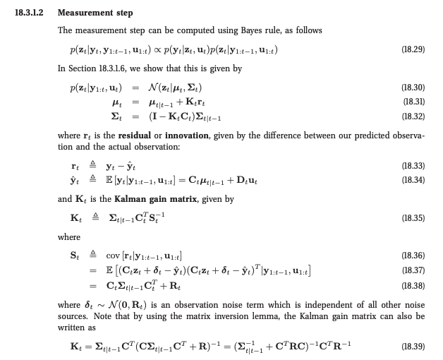
You can check out the simple implementation in the notebook. Here are the filtered values we get for $\mathbf{z}_t$:
Kalman filters tend to be quite robust to getting the parameters a bit wrong. Which is good since you don’t always know the parameters exactly. Here’s the filtering with the following parameters:
params["A"] = 0.4       # actual 0.9
params["B"] = 3         # actual 2
params["Q"] = 4.9       # actual 2.0
params["C"] = 1         # actual 1.0
params["D"] = -1        # actual -1
params["R"] = 6         # actual 4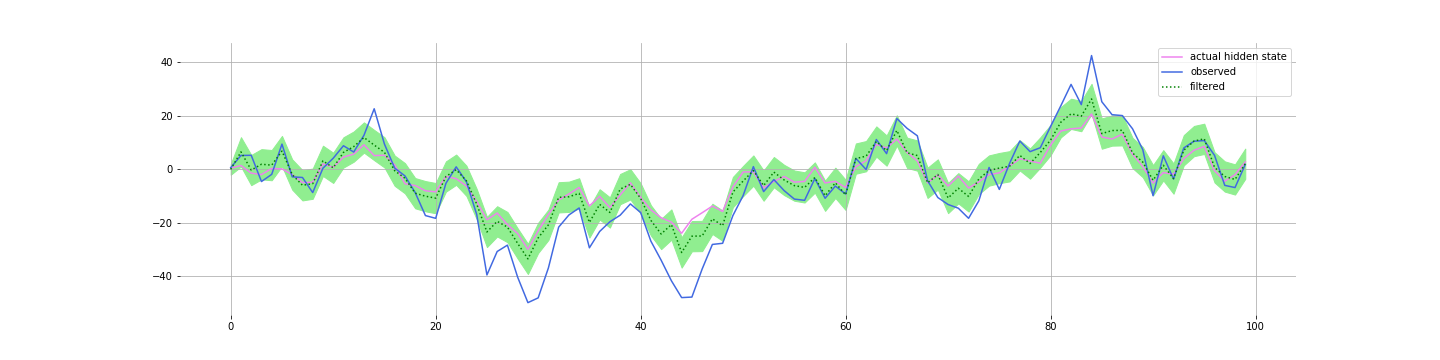
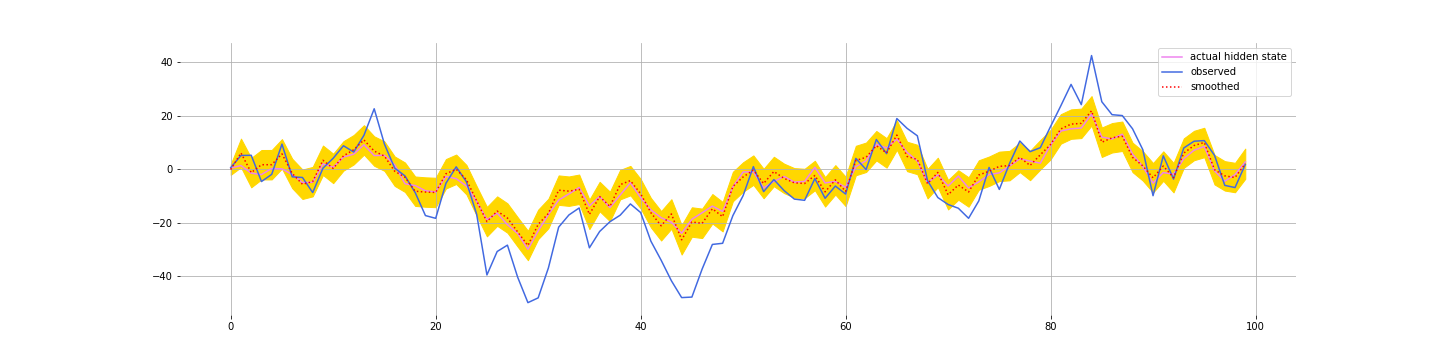
And if you are smoothing (using data filter for all time periods, $T$, to estimate the value for time $t$), then you do even better:
PYMC3 to infer parameters
PYMC3 has some time-series methods implemented for you. If you squint, the hidden process $\mathbf{z}_t$ is pretty similar to the an $AR1$ process. The only difference is that instead of:
\[z_{t + 1} = A z_t + \epsilon_t\]we have:
\[z_{t + 1} = A z_t + B u_t + \epsilon_t\]So let’s just modify the $AR1$ implementation for this change:
class LinearGaussianSSM(pm.distributions.distribution.Continuous):
    """
    Linear Gaussian SSM with 1 lag.
    Parameters
    ----------
    k: tensor
       effect of lagged value on current value
    tau_e: tensor
       precision for innovations
    mu: tensor
       the mean shift for the process
    """

    def __init__(self, k, tau_e, mu, *args, **kwargs):
        super().__init__(*args, **kwargs)
        self.k = k = tt.as_tensor_variable(k)
        self.tau_e = tau_e = tt.as_tensor_variable(tau_e)
        self.tau = tau_e * (1 - k ** 2)
        self.mode = tt.as_tensor_variable(0.0)
        self.mu = tt.as_tensor_variable(mu)

    def logp(self, x):
        """
        Calculate log-probability of LG-SSM distribution at specified value.
        Parameters
        ----------
        x: numeric
            Value for which log-probability is calculated.
        Returns
        -------
        TensorVariable
        """
        k = self.k
        tau_e = self.tau_e  # innovation precision
        tau = tau_e * (1 - k ** 2)  # ar1 precision
        mu = self.mu

        x_im1 = x[:-1]
        x_i = x[1:]
        boundary = pm.Normal.dist(0, tau=tau).logp

        innov_like = pm.Normal.dist(k * x_im1 + mu, tau=tau_e).logp(x_i)
        return boundary(x[0]) + tt.sum(innov_like)

    def _repr_latex_(self, name=None, dist=None):
        if dist is None:
            dist = self
        k = dist.k
        tau_e = dist.tau_e
        name = r"\text{ %s }" % name
        return r"${} \sim \text(\mathit={},~\mathit={},~\mathit={})$".format(
            name, get_variable_name(k), get_variable_name(tau_e), get_variable_name(mu)
        )
That’s it. Easy. Now let’s fit the model:
with pm.Model() as model:

    sig = pm.HalfNormal("σ", 4)

    alpha = pm.Beta("alpha", alpha=1, beta=3)
    sig1 = pm.Deterministic(
        "σ1", alpha * sig
    )
    sig2 = pm.Deterministic(
        "σ2", (1 - alpha) * sig
    )

    A_ = pm.Uniform("A_", -1, 1)
    B_ = pm.HalfNormal("B_", 2)
    mu = B_ * ut[1:]

    f = LinearGaussianSSM("z", k=A_, tau_e=1 / (sig1 ** 2), mu=mu, shape=yt.shape)

    C_ = pm.HalfNormal("C_", 2)
    D_ = pm.Normal("D_", 0, 2)
    y_mu = pm.Deterministic("y_mu", C_ * f + D_ * ut)

    likelihood = pm.Normal("y", mu=y_mu, sd=sig2, observed=yt)

    trace = pm.sample(1000, target_accept=0.99, tune=3000)
That splitting of the $\sigma$ is a trick I picked up from pymc3 discourse. The total variation needs to be distributed between the two levels. We’ll introduce another parameter, $\alpha$, that determines the allocation of the variation to each.
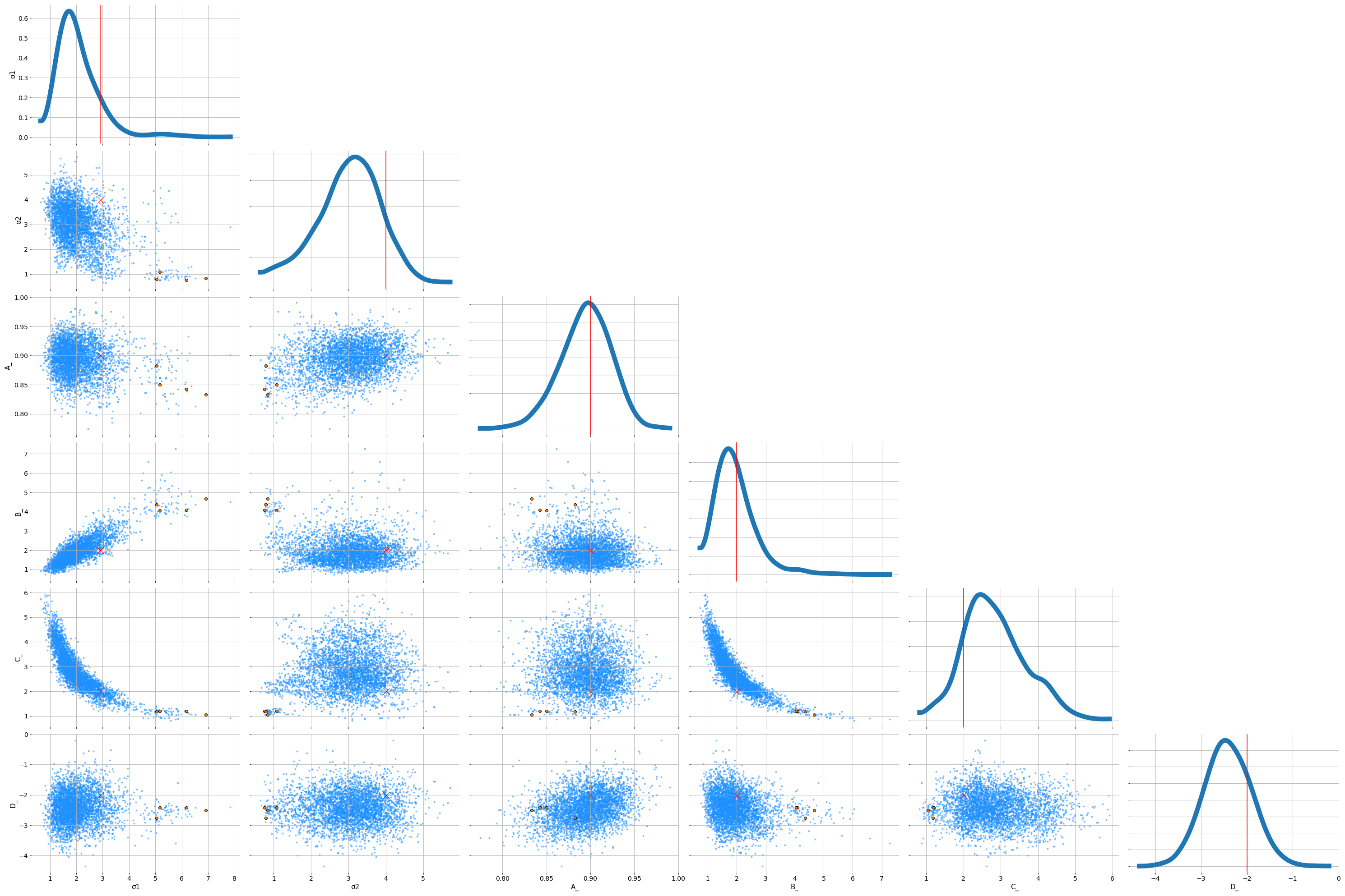
Those divergences seems to be when $\sigma 1$ gets too small. We could try other parameterisations to shake those off. Overall, we seem to have recovered the parameters pretty well.
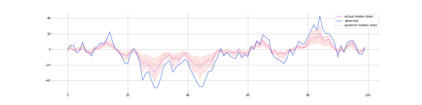
And here’s the posterior for the hidden state:
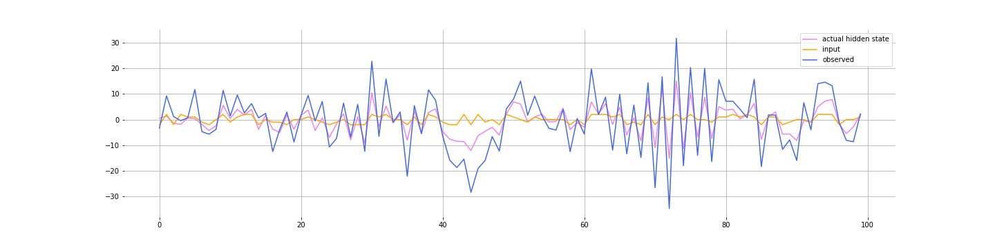
PYMC3 with non-stationary parameters
An SSM where the parameters don’t change is called stationary. Here’s one where $A$ is not static but rather changes as a cosine function.
size = 100
np.random.seed(15)

z0 = 0.5
ut = np.random.choice(np.arange(-2, 3), size=size)
zt = np.zeros(ut.shape[0])
yt = np.zeros(ut.shape[0])

A = 0.9 * np.cos(np.linspace(0, 2 * np.pi * 2, size))
B = 2
C = 2
D = 0

Q = 2.9
R = 4
for i, u in enumerate(ut):
    if i == 0:
        zt[i] = z0
    else:
        zt[i] = A[i] * zt[i - 1] + B * ut[i] + np.random.normal(0, Q)
    yt[i] = C * zt[i] + D * (ut[i]) + np.random.normal(0, R)
Here’s what the data look like:
Fitting the models
The key thing we are changing is that we are modelling $A$ as Gaussian Random Walk. So $A$ changes slowly over time.
with pm.Model() as model2:
sig = pm.HalfNormal("σ", 4)
alpha = pm.Beta("alpha", alpha=1, beta=3)
sig1 = pm.Deterministic(
"σ1", alpha * sig
)
sig2 = pm.Deterministic(
"σ2", (1 - alpha) * sig
)
A_sigma = pm.HalfNormal("A_sigma", 0.2)
A_ = pm.GaussianRandomWalk(
"A_", mu=0, sigma=A_sigma, shape=(size), testval=tt.zeros(size)
)
B_ = pm.HalfNormal("B_", 2)
mu = B_ * ut[1:]
f = LinearGaussianSSM("z", k=A_[1:], tau_e=1 / (sig1 ** 2), mu=mu, shape=yt.shape)
C_ = pm.HalfNormal("C_", 2)
D_ = pm.Normal("D_", 0, 2)
y_mu = pm.Deterministic("y_mu", C_ * f + D_ * ut)
likelihood = pm.Normal("y", mu=y_mu, sd=sig2, observed=yt)
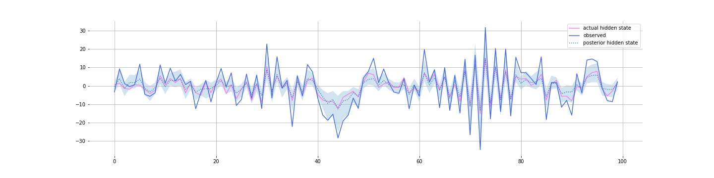
trace2 = pm.sample(1000, target_accept=0.99, tune=3000)Results
Check out the notebook. Divergences abound. Maybe you can fix it. But I just want to show you what the posterior looks like:
And most interestingly, what we learn about $A$:
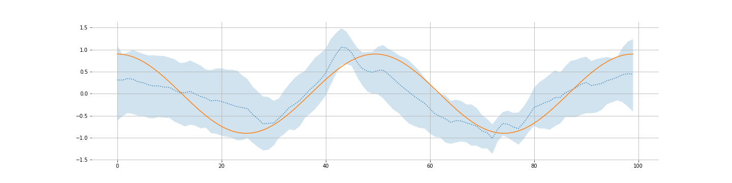
Not great but generally there.
Conclusions
When the observation error in $y_t$ and the system error in $z_t$ are both large, these models do well. If not, you can probably use a simpler model and do just fine.
The bloopers reel
Fitting these models is tricky. I was listening to Alex Andorra’s podcast. Good podcast, check it out. They often talk about how tricky these models can be. I spent a lot of time debugging divergences and failed chains. One example is if specifically telling the model that $A$ follows a cosine of some frequency. Or if you even give it the frequency but you say it follows a sine with some phase. You’d think these model would fit better. I couldn’t figure out why it doesn’t. I also tried using pm.Bound to restrict $A$ to be between -1 and 1. You’d think that would help it along. Nope - I guess gradient go funny at the edges when you use pm.Bound.
In the model above, try making C_ and B_ Normals instead of a Half Normals. You see something interesting - the posterior for these values is bimodal. And your rhat values are wild since your chains might be exploring different modes. And that makes sense. The hidden state can be the inverted as long as you are inverting the coefficient C_ as well. Obvious now in hindsight but not something I had thought about before I ran the model.
At some stage, I’d love to do a post of just my hacky failures. All those attempts to fit fancy models that came to nothing. Also, should talk about how good the pymc3 discourse it.