A colleague of mine came across an interesting problem on a project. The client wanted an alarm raised when the number of problem tickets coming in increased “substantialy”, indicating some underlying failure. So there is a some standard rate at which tickets are raised and when something has failed or there is serious problem, a tonne more tickets are raised. Sounds like a perfect problem for a Hidden Markov Model.

As per usual, you can find the notebook with all the code here.

The problem

Let’s simulate some data. We assume that there are two states of the world. The normal (n) or business-as-usual state, and snafu (s) state. We move between these states as per some transition matrix:

When things are normal, i.e. we are in n state, ticket arrivals follow a Poisson process with rate, $\lambda_n$. When it’s not, tickets follow a Poisson process with a different rate, $\lambda_s$. I wrote a utility class to make data generation easy. I won’t do into it here but you can check out the code here.

sg = SampleGenerator("poisson", [{'lambda':5}, {'lambda': 10}], 2,
                     np.array([[0.8, 0.2],[0.2, 0.8]]))

vals_simple, states_orig_simple = sg.generate_samples(100)

vals_simple has the number of tickets raised, states_orig_simple has the states. I chose $\lambda_n$ to be 5 and $\lambda_s$ to be 10. You’d imagine in real life that $\lambda_s$ would be possibly an order of magnitude higher that $\lambda_n$. But that would be too easy and no fun.

We observe just the number of tickets being raised i.e. vals_simple. So we need to recreate states_orig_sample (we’ll actually also infer $\lambda_b$, $\lambda_s$, and T along the way).

The data

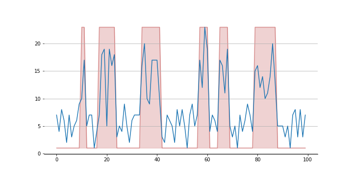
Here’s what the data looks like:

The orange dots come from the Poisson process of state s which has rate $\lambda_s$ which we chose as 10. They tend to be higher on average than the blue dots though not always. For example, timestamps 43 and 44 will be interesting to watch.

Setup the simple model

We’re going to use Pymc3 to setup our model. Let’s define some custom distributions

class StateTransitions(pm.Categorical):
    '''
    Distribution of state at each timestamp
    '''
    def __init__(self, trans_prob=None, init_prob=None, *args, **kwargs):

        super(pm.Categorical, self).__init__(*args, **kwargs)

        self.trans_prob = trans_prob
        self.init_prob = init_prob

        # Housekeeping
        self.mode = tt.cast(0,dtype='int64')
        self.k = 2

    def logp(self, x):

        trans_prob = self.trans_prob

        p = trans_prob[x[:-1]] # probability of transitioning based on previous state
        x_i = x[1:]            # the state you end up in

        log_p = pm.Categorical.dist(p, shape=(self.shape[0],2)).logp_sum(x_i)

        return pm.Categorical.dist(self.init_prob).logp(x[0]) + log_p


class PoissionProcess(pm.Discrete):
    '''
    Likelihood based on the state and the associated lambda
    at each timestamp1
    '''    
    def __init__(self, state=None, lambdas=None, *args, **kwargs):

        super(PoissionProcess, self).__init__(* args, ** kwargs)

        self.state = state
        self.lambdas = lambdas

        # Housekeeping
        self.mode = tt.cast(1,dtype='int64')

    def logp(self, x):

        lambd = self.lambdas[self.state]
        llike = pm.Poisson.dist(lambd).logp_sum(x)

        return llike

Each of these classes defines the likelihood for all the states in the entire sequence. Why the whole sequence? Say you’re in state n at time t and you observe an 8 at time t+1. Did you transition to state s for t+1 or was this just an unlikely draw from the normal n state? What if you see a 3 at time t+2? What about if you see a 12 at time t+2? This line of argument can be extended in both directions. So you need to consider all the states - one at each timestamp - at the same time.

With this defined, it’s easy to setup the model.

chain_tran = tr.Chain([tr.ordered])

with pm.Model() as m:

    lambdas = pm.Gamma('lam0', mu = 10, sd = 100, shape = 2, transform=chain_tran,  
                        testval=np.asarray([1., 1.5]))

    init_probs = pm.Dirichlet('init_probs', a = tt.ones(2), shape=2)
    state_trans = pm.Dirichlet('state_trans', a = tt.ones(2), shape=(2,2))

    states = StateTransitions('states', state_trans, init_probs, shape=len(vals_simple))

    y = PoissionProcess('Output', states, lambdas, observed=vals_simple)

The trickiest thing here to enforce that $\lambda_n$ is smaller than $\lambda_s$. You can use pm.Potential to add -np.inf to the loglikehood if the ordering is violated. That’s how I’ve done it before. But for some reason my chains seem to mix better when using the tr.ordered transform. I don’t understand the underlying geometry (or internals of pymc3) enough to explain why. Maybe I just got lucky. If you know, please drop me an email or comment below.

Let’s draw some samples.

with m:
    trace = pm.sample(tune=2000, sample=1000, chains=2)

Results of the simple model

We look at the mean of our states RV with +/- 2 standard deviations (not the best way I know but fine for our purpose).

Not too bad. We nailed most of states. We don’t get timestamp 43 right but that was always going to be tricky one.

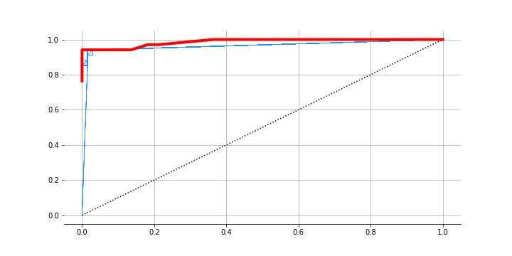
Since it is a kind of classification problem, let’s see what the ROC looks like:

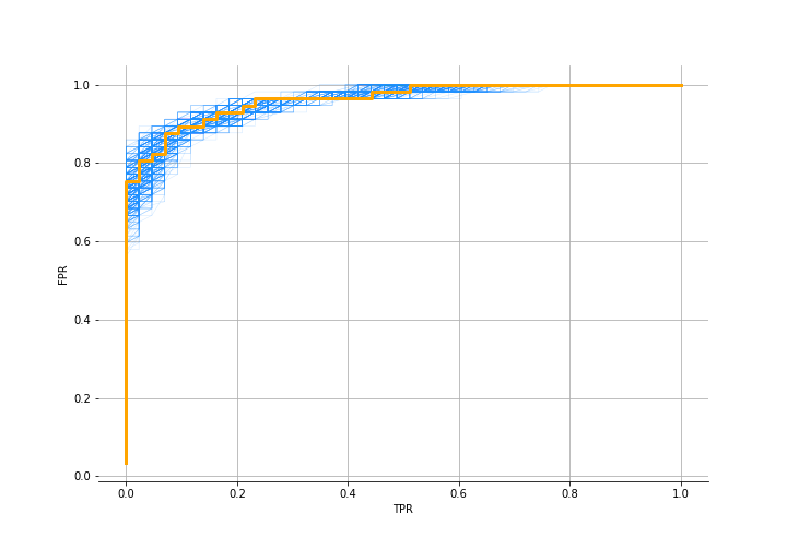
The AUC is 0.96. So we used just observations of the number of tickets and were able to infer the state we are in. Check out the notebook for more details and to see that we infer the two lambdas and the transition matrix quite well as well.

The more complex problem

The more observant readers are asking where the “hierarchical” mentioned in the title fit in. Here it is.

Say you’re pleased with the model above and go setup 10 of those for each of the different classes of tickets. Everything is humming along nicely; we’re detecting state changes early and taking action. The one day ALL 10 models raise alerts. What just happened? Well there is some overarching or common problem that exhibits as tickets for all of these classes. The classes are interconnected within some hierarchy.

So what we want to know is this: observing just the tickets for each of the 10 classes, can we identify when there is common problem that is affecting them all? I.e. there is a higher level process that has changed state. And, it affects the number of tickets observed in each of the 10 classes, regardless of what state they are in themselves (so really, there are 4 states based on the combinations of possible states of the super process and sub-process: nn, ns, sn, ss).

Let’s simulate this higher level process.

n_samples = 100
n_cats = 12

sg3_super = SampleGenerator("poisson", [{'lambda':5}, {'lambda': 15}], 2,
                     np.array([[0.9, 0.1],[0.1, 0.9]]))
vals_super, states_orig_super = sg3_super.generate_samples(n_samples)

We chose lambdas as 5 and 15. Far enough that it should be easier to infer the states if we were actually given val_super.

For each of the classes or sub-processes, we have 12 of them here, let’s generate some tickets and states:

vals = np.zeros((n_cats, n_samples))
vals_h = np.zeros((n_cats, n_samples))

stages = np.zeros((n_cats, n_samples))
for sim in range(n_cats):

    s1 = sp.stats.dirichlet.rvs(alpha=[18, 2])
    s2 = sp.stats.dirichlet.rvs(alpha=[2, 18])
    transition = np.stack([s1, s2], axis=1).squeeze()

    sg = SampleGenerator("poisson", [{'lambda':5}, {'lambda': 10}],
                         2, transition)

    vals[sim, :], stages[sim, :] = sg.generate_samples(n_samples)
    vals_h[sim, :] = vals[sim, :] + vals_super

We keep the lambdas as 5 and 10 as in the previous simulation. vals_h is all we observe. We need to recreate the higher process states states_orig_super using these values.

The hierarchical data

Here’s what the “super” state process looks like:

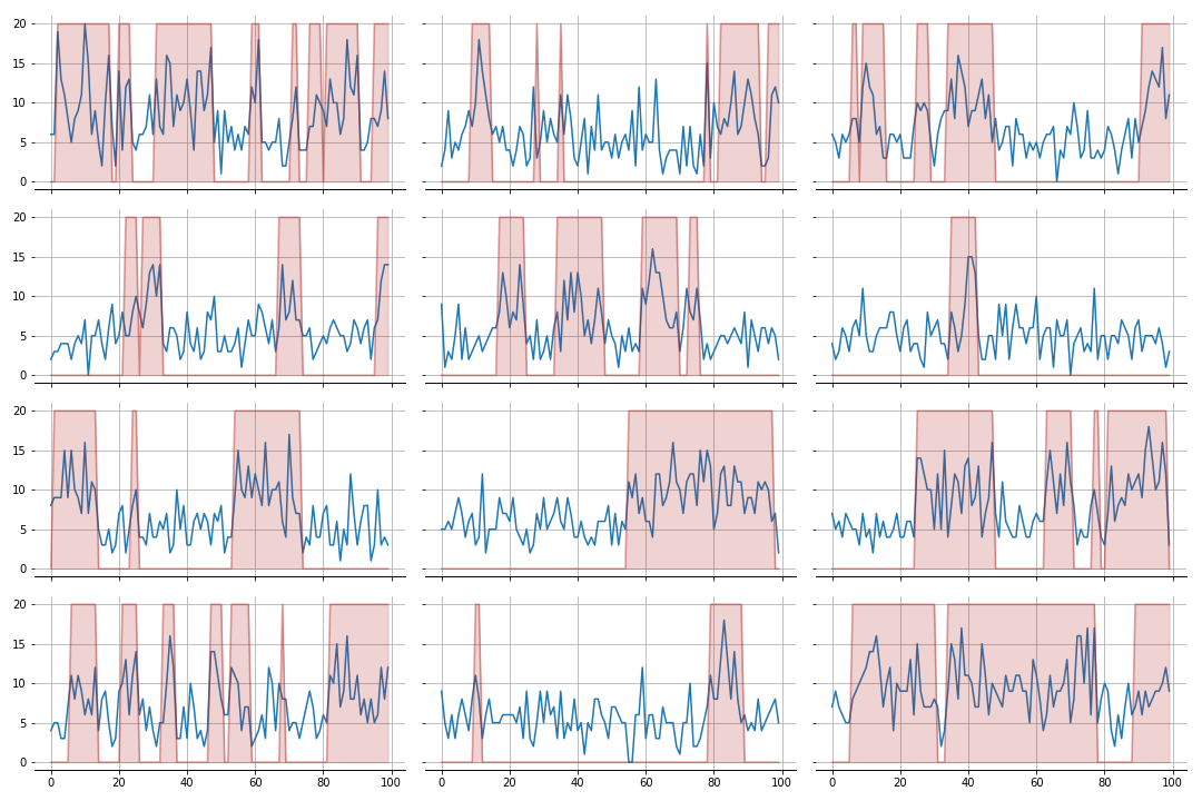
The values generated (in blue) get added to each of the sub processes you’ll see below. The 12 sub processes look like this:

Setup the hierarchical model

Here are classes again. The state transitions class is exactly the same. In the poisson process class, HPoissionProcess, we now have a mixture of two Poissons. One for the super process and one for the sub process.

class HStateTransitions(pm.Categorical):

    def __init__(self, trans_prob=None, init_prob=None, *args, **kwargs):

        super(pm.Categorical, self).__init__(*args, **kwargs)

        self.trans_prob = trans_prob
        self.init_prob = init_prob

        # Housekeeping
        self.mode = tt.cast(0,dtype='int64')
        self.k = 2

    def logp(self, x):

        trans_prob = self.trans_prob

        p = trans_prob[x[:-1]] # probability of the previous state you were in
        x_i = x[1:]            # the state you end up in

        log_p = pm.Categorical.dist(p, shape=(self.shape[0],1)).logp_sum(x_i)
        initlike = pm.Categorical.dist(self.init_prob).logp(x[0])

        return log_p + initlike

class HPoissionProcess(pm.Discrete):

    def __init__(self, state=None, state_super=None, lambdas=None, super_lambdas=None, *args, **kwargs):

        super(HPoissionProcess, self).__init__(*args, ** kwargs)

        self.state = state
        self.super_state = state_super
        self.lambdas = lambdas
        self.super_lambdas = lambdas

    def logp(self, x):

        lambd = self.lambdas[self.state]
        lambd_super = self.super_lambdas[self.super_state]

        #llike = pm.Poisson.dist(lambd + lambd_super).logp_sum(x) # since they are independant
        llike = pm.Mixture.dist(w=[0.5, 0.5], comp_dists=[pm.Poisson.dist(lambd),
                                                          pm.Poisson.dist(lambd_super)]).logp_sum(x)

        return llike

Note that we set the mixture weights to be 0.5 and 0.5. But you could just throw a dirichlet prior on this and let it figure out what the “influence” of the super process is on the sub process. Though this would mean it would mean there are additional free parameters to learn.

Let’s setup the model.

chain_tran = tr.Chain([tr.ordered])
with pm.Model() as m2:

    lambd = [0] * n_cats
    state_trans = [0] * n_cats
    states = [0] * n_cats
    y = [0] * n_cats
    init_probs = [0] * n_cats

    lambd_super = pm.Gamma('lam_super', mu = 10, sd = 10, shape=2, transform=chain_tran,  testval=np.asarray([1., 1.5]))
    init_probs_super = pm.Dirichlet('init_probs_super', a = tt.ones(2), shape=2)
    state_trans_super = pm.Dirichlet('state_trans_super', a = tt.ones(2), shape=(2,2))
    states_super = HStateTransitions('states_super', state_trans_super, init_probs_super, shape=len(vals_super))

    for sim in range(n_cats):

        lambd[sim] = pm.Gamma('lam{}'.format(sim), mu = 10, sd = 10, shape=2,
                              transform=chain_tran, testval=np.asarray([1., 1.5]))
        init_probs[sim] = pm.Dirichlet('init_probs_{}'.format(sim), a = tt.ones(2), shape=2)
        state_trans[sim] = pm.Dirichlet('state_trans{}'.format(sim), a = tt.ones(2), shape=(2,2))
        states[sim] = HStateTransitions('states{}'.format(sim), state_trans[sim], init_probs[sim], shape=n_samples)
        y[sim] = HPoissionProcess('Output{}'.format(sim), states[sim], states_super, lambd[sim], lambd_super, observed=vals_h[sim])

That’s whole bunch of parameters we are learning. And it took around 2 hrs to run. Even at the end, there were a tonne of divergences. Since I don’t really care about the exact distribution and some approximate values of the state probabilities is sufficient, I’m going to choose to ignore them. Yes - it still does make me feel all icky inside.

Results of the hierarchical model

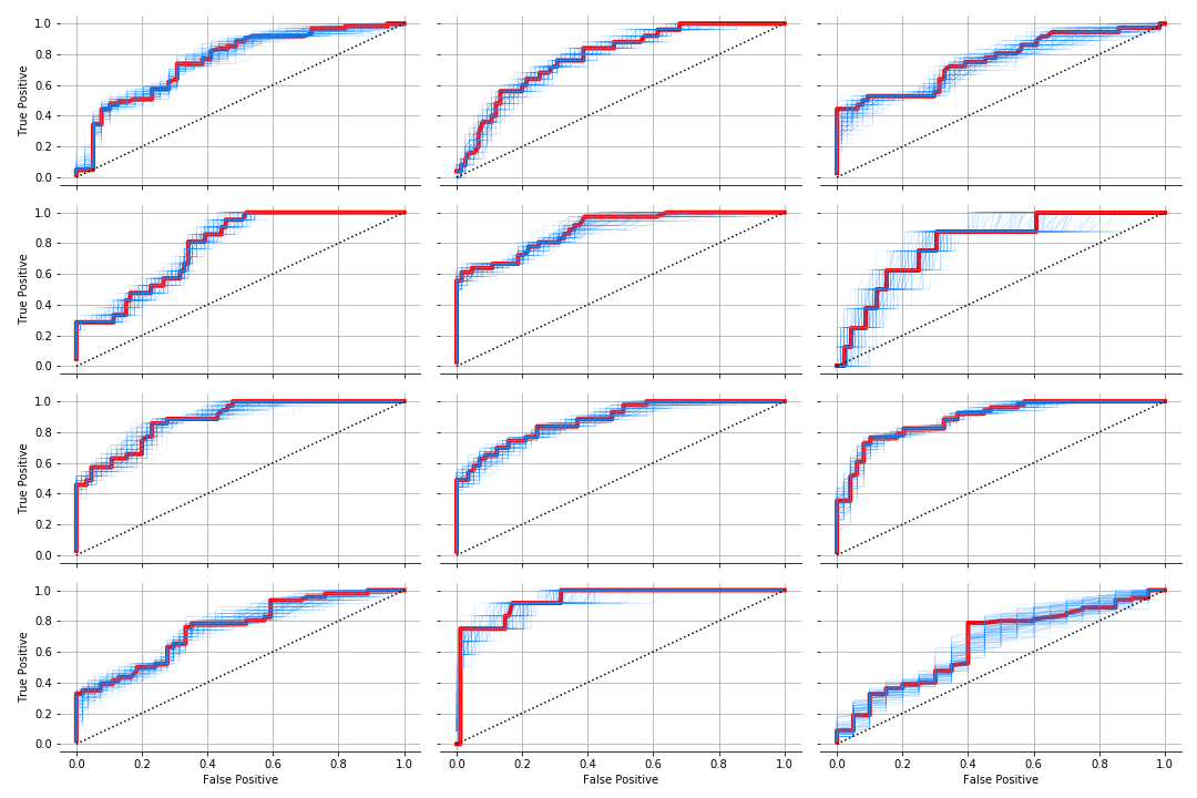
Let’s see how we do with the sub-processes first.

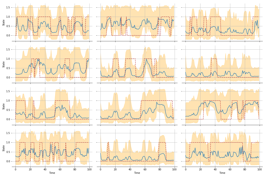
Not fantastic. The ROCs agree. We are not quite nailing it as we did earlier but it does an ok job of identifying state for most of them.

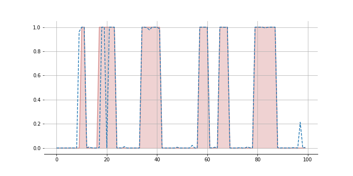
How do we do with the super process? Here’s the mean of the posterior of the states. We get a few things wrong but overall pretty decent.

Final words

Why do we do such a poor of identifying the sub-processes? We have 100 observations for each sub-process, same as the simple model, but there are more degrees of freedom since it is a mixture of two processes. Maybe we’d do better if we have had a larger sample size to train the model? Or maybe we should just train two models - a ‘simple’ HMM for each of the sub-processes and then a ‘hierarchical’ one for the super-process. Though I do like the cleanliness of having just one model and if the data-generating process is indeed hierarchical, it would perform better. But before deciding on a model, you’d want to do some model checking to see how well the hierarchical one fits your data.

I tried a few different parameterizations for the mixture model but none seem to resolve the divergences. Would love to hear from you if you have any suggestions for this.

Last thing, in IRL the world is changing underneath your feet. In our model, we assumed that the transition matrix is fixed at all times but you can imagine one that gradually drifts. We may want to model it as time-varying. Also, you may want to model the stage n process as a zero-inflated Poisson. It fits the data a lot better. Many days there are no tickets but when there are, there are a bunch.

Finally, I found this repository quite useful when building these models. So a lot of the credit should go to Mr. Strey. You can find my notebook with these results here. Thanks for reading.