You'll be blown a way by this weird trick millennials discovered to do convergence regressions.

Hat tip to @mkessler_DC for the clickbaitey title.

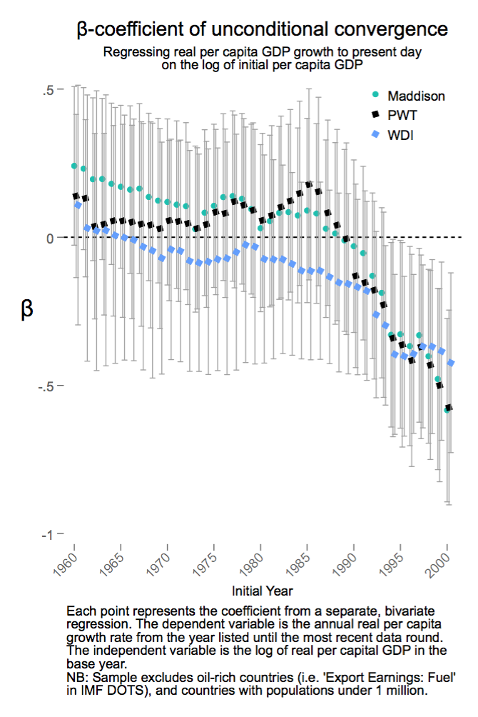
So economic convergence is back. Dev Patel, Justin Sandefur, and Arvind Subramanian (PSS) recently wrote a blog post to show that

while unconditional convergence was singularly absent in the past, there has been unconditional convergence, beginning (weakly) around 1990 and emphatically for the last two decades.

They do a very straightforward analysis; they regress real per capita GDP growth rate on the log of per capita GDP for various periods and show that the coefficient is indeed reducing. They also made their code available, which is so awesome that they can be forgiven for it being in STATA. Instead of doing separate regressions for each time period, I redo their analysis as a rolling regression where we allows the coefficients to change over time.

This post borrows heavily from Thomas Weicki’s two posts on Gaussian random walks.

As per usual, you can find the notebook on github.

Why rolling regression?

Key figure in the chart is this:

So for each time period between $y$ and $y_0$, we have different coefficients as follows:

Going forward we will drop $y_0$ from the notation for clarity.

This implicit assumption here is that $\beta_{y}$ is independent from $\beta_{y + 1}$. But we know that’s not entirely true. If you gave me $\beta_{y}$, I’d expect $\beta_{y + 1}$ to be pretty similar and deviate only slightly.

We can make this explicit and put a gaussian random-walk prior on beta.

$\sigma^2$ is how quickly $\beta$ changes. It’s just a hyper-parameter that we’ll put a weak prior on. We do the same thing for $\alpha$ as well.

Pre-processing

In the notebook, I tried replicate PSS’s STATA code in python as closely as possible. It’s not perfect. And looks like I screwed up the WDI dataset manipulations so I use only Penn World Table (PWT) and Maddison Tables (MT) in this post. Check out the notebook if you want to fix it and get it working for WDI.

Here’s what 1985 looked like:

And here’s what 2005 looked like:

The trend might not be so obvious in 1985 but it does appear to be negative in 2005, especially if you ignore those really tiny countries. Let’s see what the random walk model says.

Setup in pymc3

Here’s the model in pymc3 for MT. The code for PWT is pretty identical.

with pm.Model() as model_mad:

    sig_alpha = pm.Exponential('sig_alpha', 50)
    sig_beta = pm.Exponential('sig_beta', 50)

    alpha = pm.GaussianRandomWalk('alpha', sd =sig_alpha, shape=nyears)
    beta = pm.GaussianRandomWalk('beta', sd =sig_beta, shape=nyears)

    pred_growth = alpha[year_idx] + beta[year_idx] * inital
    sd = pm.HalfNormal('sd', sd=1.0, shape = nyears)

    likelihood = pm.Normal('outcome',
                           mu=pred_growth,
                           sd=sd[year_idx],
                           observed=outcome)

• nyears is the number of years. So there are nyears alphas and betas and they are linked as per (1).
• year_idx indexed to right coefficients based on $y$.
• As in PSS, outcome is $\Delta GDPPC_{c, y, y_0}$ and intial is $log(GDPPC_{c, y0})$.

and let’s run it:

trace_mad = pm.sample(tune=1000, model=model_mad, samples = 300)

Results

Let’s see how alpha and beta change over the years.

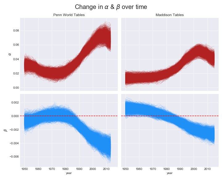
So, PSS’s conclusion is borne out here as well. We see that $beta$ used to be mildly positive and gradually shifted to negative in recent years. Our bounds look a little tighter and maybe the shape is slightly different. You can check out the notebook here. I threw this together pretty quickly so I might be screwed up the data setup. Let me know if you find any errors in my code.