Inference and EM (Baum-Welch) for HMM learning

Last month, I did a post on how you could setup your HMM in pymc3. It was beautiful, it was simple. It was a little too easy. The inference button makes setting up the model a breeze. Just define the likelihoods and let pymc3 figure out the rest.

I have been reading Murphy’s thesis for work and decided it’d be a whole lot of fun to implement the EM algorithm for learning. So here we go. The code can be found online here. Murphy’s Machine Learning book was very useful when coding up this algorithm.

Since we are going to be getting into the weeds a bit, let’s define some terms. We’re going to use the notation from Murphy’s thesis. Time goes from $1 … T$.

• $y_{1:t} = (y_1,…,y_t)$: the observations up to present time, $t$.
• $X_t$: The hidden state at time $t$.
• $P(X_t \vert y_{i:t})$: Belief state at time $t$.
• $P(X_t \vert X_{t-1})$: State-transition function. We assume we have a first-order Markov with transition matrix $A$.
• $\pi$: $P(X_1)$ - the initial state

There are a few types of inferences as per Murphy:

1. Filtering: Compute the belief state
2. Smoothing: Compute $P(X_t\vert y_{1:T})$ offline, given all the evidence.
3. Fixed lag smoothing: Slightly lagged filtering - $P(X_{t-l}\vert y_{1:t})$
4. Prediction: Predict the future - $P(X_{t+l}\vert y_{1:t}$)

We’re just going to look at the first two: filtering and smoothing. Then use some of these functions to implement an EM algorithm for learning the parameters.

Generate data

We’ll use the utility classes from the last post to generate some data:

n_samples = 100
t_mat = np.array([[0.8, 0.2],[0.2, 0.8]])
init = 0

sg = SampleGenerator("poisson", [{'lambda':5}, {'lambda': 10}],
                     2, t_mat)
vals, states_orig = sg.generate_samples(n_samples, init_state=init)

vals are all we observe.

Filtering - The forwards algorithm

Check out Murphy for the full derivation but the forward algorithm boils down to this:

where $A$ is the Markov transition matrix that defines $P(X_t \vert X_{t-1})$ and $O_t(i, i) = P(y_t \vert X_t = i)$ is a diagonal matrix containing the conditional likelihoods at time $t$.

Note that $\alpha_t$ is recursively defined with the base case being:

And here it is in python:

def forward_pass(y, t, dists, init, trans_mat):

    x0 = dists[0]
    x1 = dists[1]
    all_c = []
    if t == 0:
        O = np.diag([x0.pmf(y[0]), x1.pmf(y[0])])
        c, normed = normalize(O @ init)
        return c, normed.reshape(1, -1)

    else:
        c_tm1, alpha_tm1 = forward_pass(y, t - 1, dists, init, trans_mat)

        O = np.diag([x0.pmf(y[t]), x1.pmf(y[t])])
        c, normed = normalize(O @ trans_mat.T @ alpha_tm1[-1, :])

        return c_tm1 + c, np.row_stack([alpha_tm1, normed])

Here’s the normalize function that is called in forward_pass that we’ll use again. Pretty straightforward stuff:

def normalize(mat, axis=None):
    c = mat.sum(axis=axis)
    if axis==1:
        c = c.reshape(-1, 1)
    elif axis == 0:
        c = c.reshape(1, -1)

    return c, mat / c

Here’s what our filtered signal looks like.

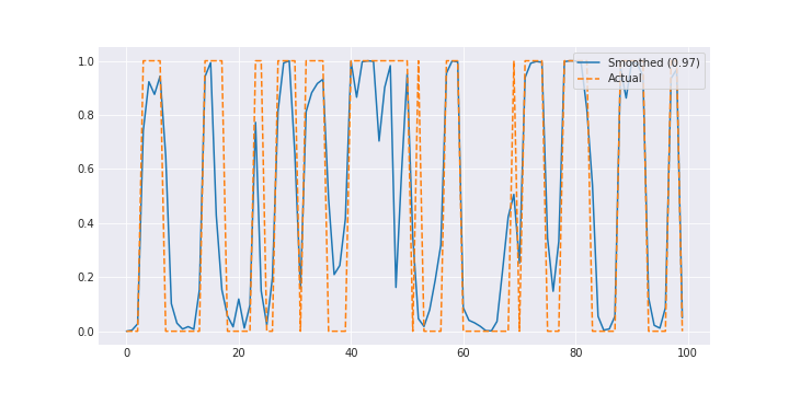
The results are pretty good. You could make the problem a little harder by making the two lambdas closer together or throwing in some noise.

Smoothing - The forwards-backwards algorithm

I like how Murphy explains why uncertainty will be lower in smoothing:

To understand this intuitively, consider a detective trying to figure out who committed a crime. As he moves through the crime scene, his uncertainty is high until he finds the key clue; then he has an “aha” moment, his uncertainty is reduced, and all the previously confusing observations are, in hindsight, easy to explain.

Here we define two new terms:

As with $\alpha$, $\beta$ is recursively defined with the base case:

Let’s code this $\beta_t$ up in python:

def backward_pass(y, T, t, dists, init, trans_mat):

    x0 = dists[0]
    x1 = dists[1]
    all_c = []

    if t == T:
        c, normed = normalize(np.ones(2))
        return 0, normed.reshape(1, -1)
    else:

        c_tm1, beta_tp1 = backward_pass(y, T, t+1, dists, init, trans_mat)
        O = np.diag([x0.pmf(y[t+1]), x1.pmf(y[t+1])])
        c, normed = normalize(trans_mat @ O @ beta_tp1[-1, :])

        return c_tm1 + c, np.row_stack([normed, beta_tp1])

and then we can put the two together to get $\gamma$:

def gamma_pass(y, T, t, dists, init, trans_mat):

    consts_f, state_prob_forward = forward_pass(y, T, dists, init, trans_mat)
    consts_b, state_prob_backward = backward_pass(y, T, t, dists, init, trans_mat)

    gamma = (state_prob_backward * state_prob_forward)

    return gamma

We were already doing quite well but this improves the AUC even further.

EM (Baum-Welch) for parameter learning

All that seems fine but we gave the algorithm $A$, $\pi$, and even the parameters associated with the two hidden states. What we learned using pymc3 last time was all of the parameters using just the observations and a few assumptions.

We’ll do that again using the EM algorithm.

Two-slice distributions

We are going to code up the two-slice distribution since it’s about to come in handy. It is defined as follows:

and Murphy shows that it can be computed as follows:

(Note: The formula in Murphy’s thesis didn’t make sense to me so this is going off his book.)

So let’s do it:

def two_slice(y, T, t, dists, init, trans_mat):

    cs, betas = backward_pass(y, T, t, dists, init, trans_mat)
    cs, alphas = forward_pass(y, t-1, dists, init, trans_mat)

    alpha = alphas[-1]
    beta = betas[0]

    O = np.diag([x0.pmf(y[t]), x1.pmf(y[t])])

    c, normed = normalize(trans_mat * (alpha @ (O * beta).T), axis=None)

    return c, normed

E-step

Ugh. There is a tonne of latex here to write. So I’m going take the easy way out and just paste it from the book. Sorry Mr. Murphy if this breaks any laws. Let me know and I’ll remove it immediately. Also, I’m a big fan of your work.

This also means that the notation is a little different. $z$ is the hidden state and $\mathbf{x}$ is the observation.

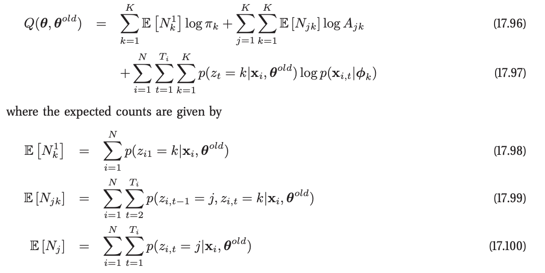
Since we only have one process, let’s just drop the summation over $N$. In code, this is:

def E_step(y, A, B, pi):

    dists = sct.poisson(B[0]), sct.poisson(B[1])

    all_gammas = gamma_pass(y, 99, 0, dists, pi, A)

    En1k = all_gammas[0]
    Enjk = reduce(lambda x,y : x+y, map(lambda t: two_slice(y, 99, t, dists, pi, A)[1], range(1, 100)))
    Enj = reduce(lambda x,y: x + y, all_gammas)

    first_term = En1k @ np.log(pi)
    middle_term = (Enjk * np.log(A)).sum()

    p_z = np.log(np.row_stack([dists[0].pmf(y), dists[1].pmf(y)]))
    final_term = (p_z * all_gammas.T).sum()

    like = first_term + middle_term + final_term

    return like, En1k, Enjk, Enj, all_gammas

Wow. Such ease. Much elegant.

M-step

This step is even easier. I won’t bother with the math, since the code is quite obvious:

def M_step(y, En1k, Enjk, Enj, all_gammas):

    A = Enjk / Enjk.sum(axis=1).reshape(-1, 1)
    pi = En1k / En1k.sum()

    B = (all_gammas * y.reshape(-1, 1)).sum(axis=0) / Enj    

    return A, np.round(B), pi

Running the EM algorithm

We just need to run the two step until we converge. EM often gets stuck at local minima so you need to be careful how you initialize the variables. Check out Murphy 17.5.2.3 for tips on how to tackle that.

np.random.seed(55)

max_iter = 100
i = 0

pi_init = np.array([0.5, 0.5]) #npr.dirichlet(alpha=[0.5, 0.5])
z_init = npr.randint(0, 2, size=n_samples)
A_init = npr.dirichlet(alpha=[0.5, 0.5], size=2)
B_init = np.array([1, 20])

# I want to keep a copy of my init vars
z = z_init.copy()
A = A_init.copy()
B = B_init.copy()
pi = pi_init.copy()

like_new = 1e10
like_old = 1e-10

print("\n A_init:{}, B_init:{}, pi_init:{}".format(A, B, pi))
print("----------------------")
while (np.abs(like_new - like_old) > 1e-5) and (i < max_iter):
    like, En1k, Enjk, Enj, all_gammas = E_step(y, A, B, pi)
    like_old = like_new
    like_new = like
    A, B, pi = M_step(y, En1k, Enjk, Enj, all_gammas)

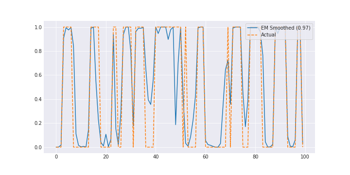
    i += 1

Check out the notebook for how it does in learning $A$, $\pi$, and the parameters for the hidden state. It’s not perfect (and of course, no credible intervals like in the bayesian case) but it’s decent.

And here’s what the smoothed signal looks like:

Conclusion

I enjoyed that a lot. Check out the notebook here. Might do a Kalman Filter one next.