Thompson Sampling and COVID testing

We’ve been doing some work with Delhi on COVID response and thinking a lot about positivity rate and optimal testing. Say you want to catch the maximum number of positive cases but you have no idea what the positivity rates are in each ward within the city but you expect wards close to each other to have similar rates. You have a limited number of tests. How do you optimally allocate these to each ward to maximise the number of positive cases you catch?

A lot of this is theoretical since IRL you are constrained by state capacity, implementation challenges, and politics ¹. But I hope that doesn’t stop you from enjoying this as much as I did.

Notebooks are up here if you want to muck around yourself.

Thompson Sampling (TS)

The problem above can be cast as a multi-armed bandit (MAB), or more specifically a Bernoulli bandit, where there are $W$ actions available. Each action $a_w$ corresponding to doing the test in a ward $w$. Reward is finding a positive case and each ward has some unknown positivity rate. We need to trade off exploration and exploitation:

• Exploration: Testing in other wards to learn their positivity rate in case it’s higher.
• Exploitation: Doing more testing in the wards you have found so far to have high positivity rates

Algorithm

TS uses the actions and the observed outcome to get the posterior distribution for each ward. Here’s a simple example with 3 wards. The algorithm goes as follows:

1. Generate a prior for each ward, w: $f_w = beta(\alpha_w, \beta_w)$ where we set $\alpha_w$ and $\beta_w$ both to 1. ².
2. For each ward, sample from this distribution: $\Theta_w \sim beta(\alpha_w, \beta_w)$
3. Let $\tilde{w}$ be the ward with the largest $\Theta$.
4. Sample in ward $\tilde{w}$ and get outcome $y_{\tilde{w}}$. $y_{\tilde{w}}$ is 1 if the sample was positive, 0 if not.
5. Update $\alpha_{\tilde{w}} \leftarrow \alpha_{\tilde{w}} + y_{\tilde{w}}$ and $\beta_{\tilde{w}} \leftarrow \beta_{\tilde{w}} + (1 - y_{\tilde{w}})$
6. Repeat 2 - 5 till whenever

For more information, see this tutorial.

A small demo

Here’s a quick simulation that shows TS in action. We have three true distributions, all with the same mean value of 0.5.

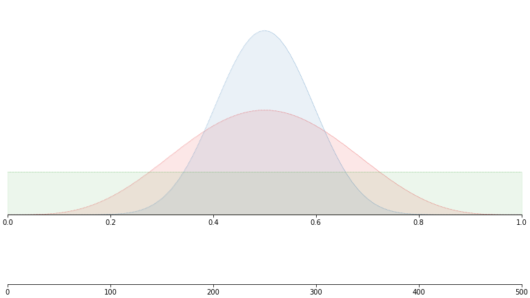
But we don’t see these. We’ll just construct a uniform prior and sample as per the algorithm above:

If you want to play around with your own distributions, check out this notebook.

Back to COVID testing

We can now do Thompson sampling to figure out which wards to test in but there is one more complication. In step 5, we update the parameters for just the ward where we sampled. But since neighbouring wards are similar, this also tells us something about those. We should really be updating their parameters as well.

How do we do that? How similar are neighbouring wards really? We’ll use our old friend gaussian processes (GPs) to non-parametrically figure this out for us.

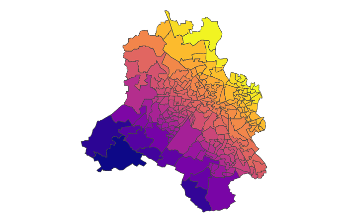
Naive estimates

For example, let’s say the true prevalence is as follows:

And we take varying number of samples - somewhere between 100 and 1000 for each - and then calculate the prevalence by just looking at number of successes / number of trials.

df['trials'] = np.random.randint(100, 1000, size= df.actual_prevalence.shape[0])
df['successes'] = st.binom(df.trials, df.actual_prevalence).rvs()
df['success_rate'] = df['successes'] / df['trials']

We end up with something looking like this:

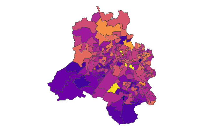
Pretty noisy. There is that general trend of high positivity in the north east but it’s not that obvious.

Gaussian Smoothing

I won’t go into the theory of GPs here. Check out these previous posts is you are interested:

1. Gaussian Process Regressions
2. Latent GP and Binomial Likelihood

In brief, we assume that wards with similar latitude and longitude are correlated. We let the model figure out how correlated they are.

Let’s setup the data:

X = df[['lat', 'lon']].values

# Normalize your data!
X_std = (X - X.mean(axis = 0)) / X.std(axis = 0)
y = df['successes'].values
n = df['trials'].values

and now the model:

with pm.Model() as gp_field:

    rho_x1 = pm.Exponential("rho_x1", lam=5)
    eta_x1 = pm.Exponential("eta_x1", lam=2)

    rho_x2 = pm.Exponential("rho_x2", lam=5)
    eta_x2 = pm.Exponential("eta_x2", lam=2)

    K_x1 = eta_x1**2 * pm.gp.cov.ExpQuad(1, ls=rho_x1)
    K_x2 = eta_x2**2 * pm.gp.cov.ExpQuad(1, ls=rho_x2)

    gp_x1 = pm.gp.Latent(cov_func=K_x1)
    gp_x2 = pm.gp.Latent(cov_func=K_x2)

    f_x1 = gp_x1.prior("f_x1", X=X_std[:,0][:, None])
    f_x2 = gp_x2.prior("f_x2", X=X_std[:,1][:, None])

    probs = pm.Deterministic('π', pm.invlogit(f_x1 + f_x2))

    obs = pm.Binomial('positive_cases', p = probs, n = n, observed = y.squeeze())

Note that we are fitting two latent GPs - one for latitude and one for longitude. This assumes that they are independent. This might not true in your data but it’s a fine approximation here.

Now we sample:

trace = pm.sample(model = gp_field, cores = 1, chains = 1, tune = 1000)

Let’s see what our smooth estimates look like:

That’s not bad at all. You can run your mouse over and see the three figures. Note how close the smooth estimates are to the actual values.

What’s next

We aren’t quite done yet but I’ll leave the rest to the reader. We need to draw from the posterior distributions we just generated and sample again. And since we used Bayesian inference, we actually have a posterior distribution (or rather samples from it) to draw from.

GPs take a lot of time fit since they involve a matrix inversion (see other post). This took me ~30 mins to sample. Even if you were doing this for realz, this might not be such a deal breaker - doubt you’re looking to come up with new testing strategies every 30 mins.

The notebook for this is up here if you’d like to play around with it yourself. Thanks for reading.

Footnotes

¹ And random sampling, and actually finding the people, and so many other thing. Also, note that positivity rate is not fixed and will change over time as you catch more positive cases and as the environment changes. We’re getting into the realm of reinforcement learning so will ignore that for now.

² You will note that this is a uniform distribution. We’re using this for simplicity but it is obviously not the right one. We don’t think wards are equally likely to have a 90% and a 10% positivity rate.