Latent GP and Binomial Likelihood

I did a quick intro to gaussian processes a little while back. Check that out if you haven’t.

I came across this presentation by Chris Fonnesbeck delivered just a few days back at PyCon 2018 on Bayesian non-parametric models. I found the idea of modeling latent variables using a Gaussian process (GP) very intriguing (and cool). We know that the latent variable has some non-linear form so instead of guessing what it might be, we can just model it using a GP.

You can get the notebook with all the code to generate the charts and the analysis here.

Moving on from a linear model

In chapter 10 of Statistical Rethinking, McElreath looks at the UC Berkeley graduate school admittance rate for men and women in a 6 departments. He models the admission rate as $logit(p_i) = \alpha_{DEPT[i]} + \beta_m m_i$. Note that he is modeling the latent variable as a linear function.

Here, we look at a similar dataset but model the latent variable as a GP using pymc3.

The data and the question

We’ll use this census data from 1994 but only look at some of the features. We want to look at the wages for men and women at different ages.

The key outcome variable of interest is >50k i.e. how many people earn over 50k given the other parameters. Or, what percent of people in a given demographic earn over 50k. The other variable of interest are: age, edu, and sex. There are other interesting variables that you may want to use to extend this model such as race, sector, and marital status but we’ll leave this out for now.

We also group edu into sensible buckets so that we end up with just 7 education groups: “Some HS”, “HS Grad”, “Some College”, “Prof School”, “Bachelors”, “Masters”, “Doctorate”.

Take 1: Using just age

Let’s ignore education for now. We’ll come back to it in the next section.

The correlation assumption

In ‘Take 1’, we use just the age and sex variable and park education for the next section. By using a GP, we assume that the probability of earning over 50k at age $x$ and $x + k$ are correlated. The closer they are (the smaller $|k|$ is), the more correlated they are. We’ll use the RBF kernel to do this since we expect it to change smoothly.

Modeling in pymc3

For each sex, we model the latent variable as a GP with pooled hyper-parameters. So the model is as follows:

with pm.Model() as admit_m:
    rho = pm.Exponential('ρ', 1)
    eta = pm.Exponential('η', 1)

    K = eta**2 * pm.gp.cov.ExpQuad(1, rho)

    gp1 = pm.gp.Latent(cov_func=K, )
    gp2 = pm.gp.Latent(cov_func=K)

    f = gp1.prior('gp_f', X=f_age)
    m = gp2.prior('gp_m', X=m_age)

    pi_f = pm.Deterministic('π_f', pm.invlogit(f))
    pi_m = pm.Deterministic('π_m', pm.invlogit(m))

    earning_f = pm.Binomial('female_over50k', p = pi_f, n=f_n.astype(int),
                           observed=f_over50k.astype(int))
    earning_m = pm.Binomial('male_over50k', p = pi_m, n=m_n.astype(int),
                           observed=m_over50k.astype(int))

Easy enough. Now let’s draw a bunch of samples and see what $p$, the probability of earning over 50k, looks like for the two sexes.

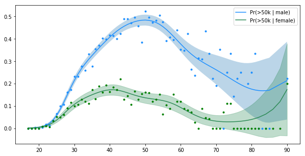
So it appears that the gap between the wages of men and women starts pretty early on and is the widest around the age of 50. Also interesting to note is that the peak for men is at 50 years while for women it’s around 40 years.

But we know that education makes a different. Maybe we just have a bunch of highly educated men in this sample so it makes sense that they would earn more.

Take 1: Using age and education

Now we include education.

The correlation assumption

In addition to the ‘correlation across ages’ assumption we made above, we also assume that the effect of education is correlated i.e. effect of “Masters” is closer to the effect of “Bachelors” than to “Some HS”.

We are also assuming one other thing: effect of education is the same across age groups and the effect of age is the same for all levels of education i.e. those two are independent. This doesn’t sound unreasonable though you can come up with reasons why this might not be true. We can get even smarter and say the education and age together are correlated but we’ll leave that for you to work out.

Modeling in pymc3

with pm.Model() as admit_m:
    rho = pm.Exponential('ρ', 1)
    eta = pm.Exponential('η', 1)

    rho_edu = pm.Exponential('ρ_edu', 1)
    eta_edu = pm.Exponential('η_edu', 1)

    K = eta**2 * pm.gp.cov.ExpQuad(1, rho)
    K_edu = eta_edu**2 * pm.gp.cov.ExpQuad(1, rho_edu)

    gp1 = pm.gp.Latent(cov_func=K)
    gp2 = pm.gp.Latent(cov_func=K)
    gp_edu = pm.gp.Latent(cov_func=K_edu)

    f = gp1.prior('gp_f', X=age_vals)
    m = gp2.prior('gp_m', X=age_vals)
    edu = gp_edu.prior('gp_edu', X=edu_vals)

    pi_f = pm.Deterministic('π_f', pm.invlogit(f[f_age_idx] + edu[f_edu_idx]))
    pi_m = pm.Deterministic('π_m', pm.invlogit(m[m_age_idx] + edu[m_edu_idx]))

    earning_f = pm.Binomial('female_over50k', p = pi_f, n=f_n.astype(int),
                           observed=f_over50k.astype(int))
    earning_m = pm.Binomial('male_over50k', p = pi_m, n=m_n.astype(int),
                           observed=m_over50k.astype(int))

Note that it is a very similar model and took me ~22 minutes to run on a oldish MacBook Pro. You might remember that GP is a ‘small data’ technique. It involves inverting matrices that is computationally quite expensive.

Now let’s look at how this varies across education level:

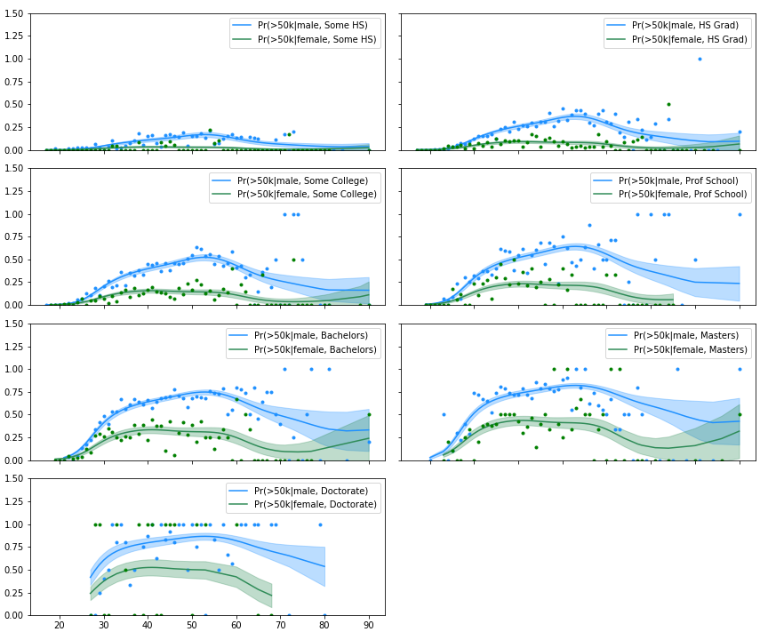
We see a wage gap in all levels of education. In the lowest categories, the gap in absolute terms is not great but in relative terms it’s yuge! The ‘plateauing’ effect for women is also interesting. The probability of earning over 50k doesn’t increase by much after mid-30s/40s for women.

Note that the relationship with age is not linear in any sense. It looks like a quadratic… maybe. If you’re a classical economist, you’re sure it’s quadratic, we’re talking about age after all, but it’s nice being agnostic.

Let’s look at the mean probability of earning over 50k in our model as a heat map.

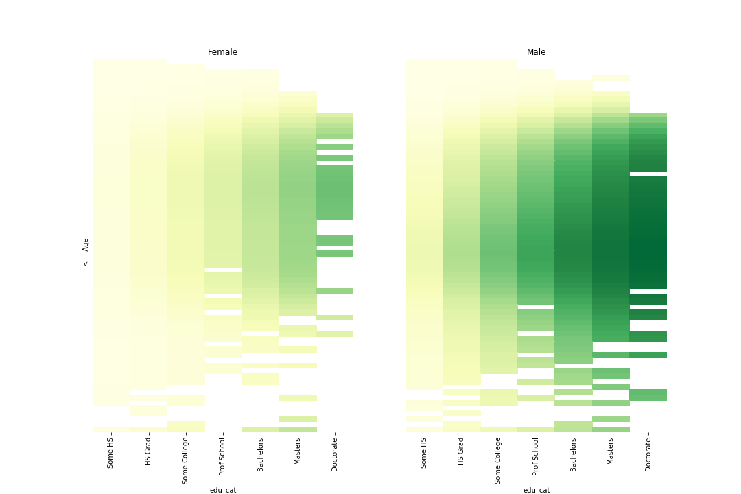
Darker cells represent higher probability of earning over 50k. Note that we are only showing the mean values here. Since we’re all Bayesian, we have the full distribution here and can show any statistics we like. Also, we noted above that there is large variation in higher ages so we should keep that in mind.

What’s with the gaps? Well, we had no data for those cells (e.g. there are no 90 year old women with Doctorates in our datasets). But fear not, we can use the model we have trained to predict it for those cells.

age_m = samples['gp_m']
age_f = samples['gp_f']
edu_gp = samples['gp_edu']

female_pp = np.zeros((len(age_vals),len(edu_vals),2000))
male_pp = np.zeros((len(age_vals),len(edu_vals),2000))

for i in tqdm(range(len(age_vals))):
    for j in edu_vals:
        female_pp[i,j,:] = pm.invlogit(age_f[:,i].reshape(-1,1) + edu_gp[:,j].reshape(-1,1)).eval().T
        male_pp[i,j,:] = pm.invlogit(age_m[:,i].reshape(-1,1) + edu_gp[:,j].reshape(-1,1)).eval().T

And plotting this:

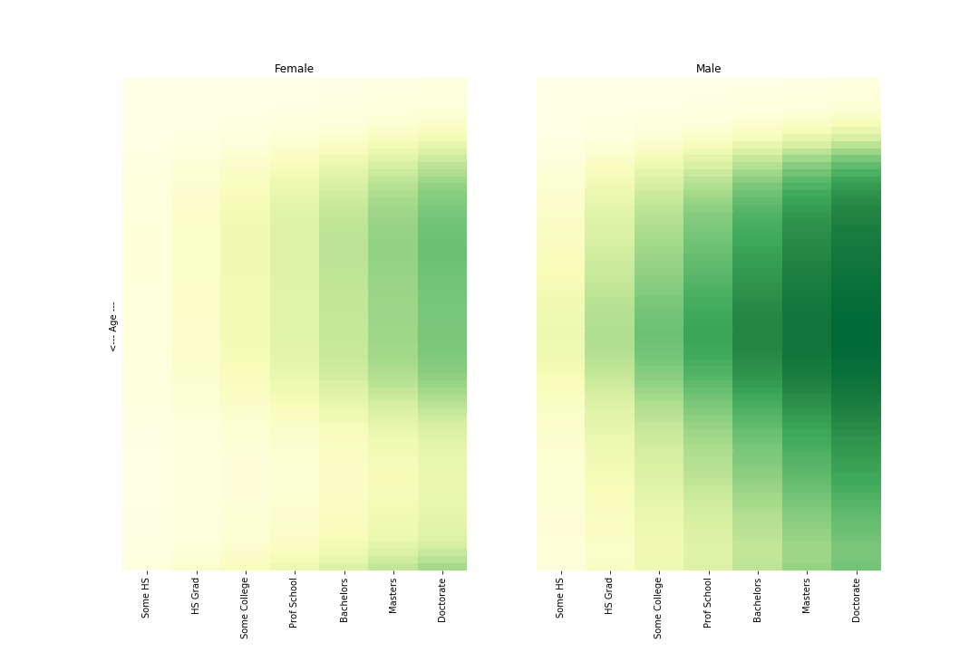
There is just more dark green for men. The earning gap exist everywhere. Unless, maybe, if you’re a kid. Anyone got a dataset of lemonade stand revenues for boys vs. girls?