This post is an intro to Gaussian Processes.
A large part of the code and explanation is borrowed from the course website for AM207 at Harvard. The notebook with the code to generate the plots can be found here.
Why Gaussian Processes
You are all probably familiar with linear regression. Since we are all bayesian, this can be written as follows:
\[\begin{aligned} y &= f(X) + \epsilon & \epsilon &\sim N(0, \sigma^2)\\ f(X) &= X^Tw & w &\sim N(0, \Sigma) \end{aligned}\]What we want is posterior predictive - we want the distribution of $”f(x’)$ as a new point $x’$ given the data i.e. $p(f(x’)|x’, X, y)$. This is a normal distribution:
\[p(f(x') | x' , X, y) = N(x'^T\Sigma X^T(X\Sigma X^T + \sigma^2 I)^{-1}y, x'^T\Sigma x' - x'^T\Sigma X^T(X\Sigma X^T + \sigma^2I)^{-1}X\Sigma x')\]$X$ is matrix where each column is a observation of x in the training set. This is pretty stock standard formula found in most bayesian stats books.
But this model can only express a limited family of functions - those that are linear in parameters.
Higher order functions
You say, “Easy!, I’ll just create more features”. You do a feature space expansion that takes $x$ and maps it to a polynomial space:
\[\phi(x) = \{x, x^2, x^3\}\\ f(x) = \phi(x)^Tw\]and sure enough, you’d do better. The posterior predictive though has a very similar structure to the linear basis example above:
\[\begin{equation} p(f(x') | x' , X, y) = N(\sigma'^T\Sigma \Phi^T(\Phi\Sigma \Phi^T + \sigma^2 I)^{-1}y, \phi'^T\Sigma \phi' - \phi'^T\Sigma \Phi^T(\Phi\Sigma \Phi^T + \sigma^2I)^{-1}\Phi\Sigma \phi') \end{equation}\]But if you mapped to an even higher polynomial space, you’d probably do even better. Actually, if you used did an infinite basis function expansion, where $\phi(x) = {x, x^2, x^3, …}$ then it can be shown that you can express ANY function (your spider sense should pointing you toward Taylor polynomials). But as you might have guessed, mapping it to high-dimensional space and then taking all those dot products would be computationally expensive. Enter the kernel trick.
The kernel trick
A kernel defines a dot product at some higher dimensional Hilbert Space (fancy way of saying it possess an inner product and has no “holes” in it). So instead of mapping your $X_1$ and $X_2$ to some high-dimensional space using $\phi(X)$ and then doing a dot product, you can just use the kernel function $\kappa(X_1, X_2)$ to directly calculate this dot product.
In the posterior for the bayesian linear regression we can just replace all those high-dimensional dot products (see equations above) with a kernel function:
\[\begin{equation} p(f(x') | x' , X, y) = N\left(\kappa(x',X) \left(\kappa(X^T,X) + \sigma^2 I\right)^{-1}y,\,\,\, \kappa(x',x') - \kappa(x',X^T)\left(\kappa(X^T,X) + \sigma^2 I\right)^{-1} \kappa(X^T,x')\right) \end{equation}\]Where:
\[\kappa(x_1, x_2) = \phi(x_1)^T \Sigma \phi(x_2)\]There are some properties that make a function a kernel - should be symmetric and the resulting Gram matrix (read: covariance matrix) should be positive definite but we won’t go into it here.
The fun bit is that some kernels (see Mercer’s Theorem) can be used to represent a dot product in an infinite space! As we discussed above, this means we can express any functional form. A radial basis function (RBF) is one such kernel:
\[\kappa(x_i, x_j) = \sigma_f^2 exp( \frac{-(x_i-x_j)^2}{2l^2})\]Where $l$ and $\sigma$ are tuning parameters that control the wiggle and the amplitude.
Though there are a number of kernels found in the wild, for the rest of this post we’ll use the RBF kernel. Mainly because Gaussians have some lovely properties that we’ll touch on later.
Enter Gaussian processes
With a kernel up our sleeve, we abandon the idea of finding weights, $w$, since there are an infinity of them anyway. Instead, we’ll think of choosing from a infinite set of functions with some mean and some covariance. So now:
\[f(x) \sim GP(m(x), \kappa(x, x'))\]Random functions
For an RBF kernel, each of the $N$ points has a normal distribution around it and can be said to be drawn from an $N$-dimensional multivariate normal distribution with a covariance defined by our kernel. So all we need to do is draw a bunch of point from this multivariate normal.
Let’s see what these look like as we vary $l$ and $\sigma$.
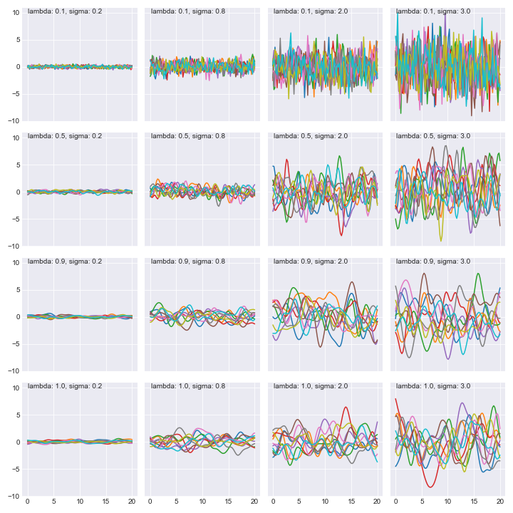
These are 10 samples from the the family of functions we’ll choose from. Exciting!
Tying it down.
Once we have some data, we can refine this infinite set of functions into a smaller (but still infinite) set of functions. How do we do that?
We want $p(f|y)$ where $y$ is the data we have observed and $f$ the set of functions. How do we calculate this posterior distribution? Here’s where Gaussian magic makes life easy. Let’s talk a little more bout these spells.
Properties of Gaussians.
Some of these are obvious and others may take some convincing. You can either do the math yourself or look it up. Though the math convinced me it didn’t really build intuition. If you’re the same, draw a bunch of samples using numpy from a multivariate normal with some covariance and plot the 3 distributions below. Once you’ve built up the intuition, go back and review the math to understand how the mean and variance is derived.
Joint of a Gaussian
A joint of a Gaussian is a Gaussian:
\[p(y,f) = \mathcal{N}\left(\left[{ \begin{array}{c} {\mu_y} \\ {\mu_{f}} \\ \end{array} }\right], \left[{ \begin{array}{c} {\Sigma_{yy}} & {\Sigma_{yf}} \\ {\Sigma_{yf}^T} & {\Sigma_{ff}} \\ \end{array} }\right]\right) = \mathcal{N}\left(\left[{ \begin{array}{c} {\mu_y} \\ {\mu_f} \\ \end{array} }\right], \left[{ \begin{array}{c} {K + \sigma^2 I} & {K'} \\ {K'^T} & {K''} \\ \end{array} }\right]\right)\]Where:
\[K' = \kappa(y, f)\\ K'' = \kappa(f, f)\\ K = \kappa(y, y)\]Marginal of a Gaussian
A marginal of a Gaussian is again a Gaussian:
\[p(f) = \int p(f,y) dy = \mathcal{N}(\mu_f, K'')\]Conditional of a Gaussian
A conditional of a Gaussian is (surprise) also a Gaussian:
\[p(f \mid y) = \mathcal{N}\left(\mu_f + K'(K + \sigma^2 I)^{-1}(y-\mu), \,\, K''-K'(K + \sigma^2 I)^{-1}K'^T \right)\]This is pretty handy. Note that the conditional is just the posterior - the family of functions $f$ given the $y$.
Calculate the posterior
Let’s say we want a Gaussian Process that can match a bunch of points (Side note: In the notebook I try to use a 20th order polynomial with to model it… and fail. We need a much higher order mapping and that gets computationally expensive).
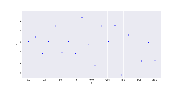
These were generated from:
\[f(x) = x^{\frac{1}{2}} \cdot sin(\frac{x}{2})\]We just go ahead and calculate \(K', K, K''\) matrices and just plug them into the formula for the conditional distribution above and voila!
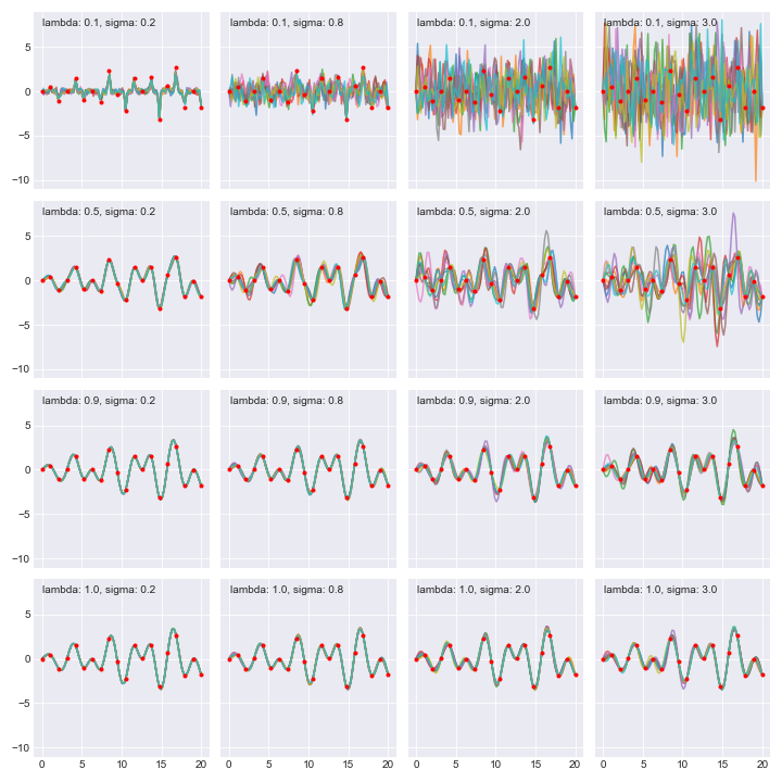
Notice how all the functions in the posterior go through our data points though what they do in between depends on $l$ and $sigma$.
Next steps
So there we have it. We fit a linear regression to a mapping of $X$ to an infinite dimensions space… by just using the RBF and its wonderful properties. One practicality that I skipped over is that we have to do a matrix inversion to calculate the posterior (or conditional). These can be computationally very expensive so this doesn’t work very well in real life if the number of data points is too large. Discovering this totally killed my buzz.
I (sort of) intentionally left all those plot up there. So which one of them is correct? How do I select $l$ and $\sigma$ parameters for the RBF? You could choose a range of them empirically and do some sort of cross validation to pick the best parameter.
Or even better: use a bayesian model. Check out the notes from this course site and Rasmussen and Williams book.
Finally, you may have noticed that we just simplified things by going with a mean of zero for both the data generating process and the model. It’s not always the best option. If your points are generally trending up, use a linear mean function.
Also, noise! I had that at the start in the formulas but then dropped it from the implementation. You should try to extend the model in the notebook to include noise.