Logit Choice Model - Estimating on a subset of alternatives

In the last two posts, we explored some features of the logit choice model. In the first, we looked at systematic taste variation and how that can be accounted for in the model. In the second, we explored one of nice benefits of the IIA assumption - we provided a random subset of alternatives of varying size to each decision maker and were able to use that to estimate the parameters.

In this post, we look at another feature of the logit model - estimating the $\beta$s using a subset of alternatives.

You can get the notebook here if you’d like to play along.

Constructing the subset

Say the decision maker chooses between $F$ different alternatives where $F$ is quite large. Estimating with that many alternative is quite hard. With a logit model, we can just use a subset of size $K$ where $K « F$. Specifically, if the decision maker chose alternative $i$ out of $F$, we can construct a smaller subset which contains $i$ and some other $K-1$ alternatives and use that for estimation.

As an example, let’s say a commuter is choosing between modes of transport to get to work. She has 100 different options like drive, walk, train, uber, canoe, … , skydive, helicopter. Say she chooses ‘canoe’, the lucky woman. We don’t need to use all the other alternatives when estimating her tastes, we can just create a subset that includes canoe. One such subset might be {canoe, walk, get a mate to drop you off}.

Uniform conditioning property

Let’s call the probability of choosing a subset $K$ given the person chose alternative $i$, $q(K \vert i)$. The following is the uniform conditioning property.

If you are picking all the other items that make up $K$ randomly, then you are are satisfying the uniform conditioning property. As your reward, you can just go ahead and estimate as we did in the previous posts where your alternatives set will be $K$ instead of $F$. This turns out to be a consistent (but not efficient) estimator of your $\beta$ parameters.

Non-uniform conditioning

Basically, $q(K \vert i) \ne q(K \vert j)\,\,\, \exists j \in K$

Why in the world would you want to do that? If most of the options are rarely ever taken (since they are terrible), picking $K$ randomly will give you subsets made up of the chosen alternative plus a bunch of highly undesirable ones. Imagine getting the following subset: {bus, hot air balloon, swim the Yarra} where $i$ is ‘bus’. If you have been anywhere near the Yarra, you know what a terrible option the last one is. You won’t learn much by observing the decision maker choose the bus over it.

One way that Train et al (1987a) get around this is by constructing the subset, $K$, based on its market share. So highly desirable options would be more likely to make it into the subset.

Adjusting the likelihood

If are going to violate the uniform conditioning property then we need to calculate $q(K \vert j)$ for all $j \in K$. This is a combinatorial problem and if $K$ is large, it going to use a few CPU cycles. If you know of clever algorithms to do this, please let me know.

Now the (conditional) likelihood is:

So we are basically augmenting the utility with the log of probability of that set being chosen.

Simulation

Let’s simulate this up with a simple example.

Setup data

Let’s setup the parameters for the simulation.

np.random.seed(31)
n_alternatives = 100     
n_params = 7              # 2^7 > 100 so we're good
n_choices = 3             # size of subset K
n_decision_makers = 1000

beta_trues = np.random.randint(-7, 7, size=n_params)

Create features for the alternatives. I’m keeping them all binary here (either the alternative has that feature or it does not) to keep it simple. Note that the option 0 is our outside option that’ll give zero utility.

all_alternative_features = []
for i in range(n_alternatives):
    features = map(int, np.binary_repr(i, width = n_params))
    all_alternative_features.append(list(features))

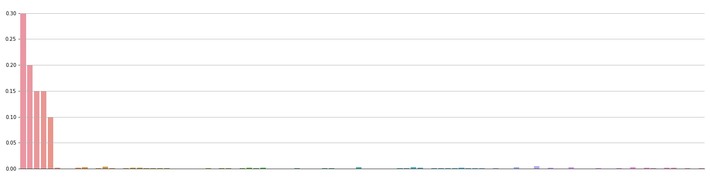
all_alternative_features = np.vstack([np.zeros((1, n_params)), np.random.permutation(all_alternative_features[1:])])

Let’s make up some market shares. The first 5 will be “significant” and then rest are tiny.

main_shares = np.array([0.3, 0.2, 0.15, 0.15, 0.1])
other_shares = np.random.dirichlet(np.ones(n_alternatives - 5), size=1).squeeze() * 0.1

market_shares = np.hstack((main_shares, other_shares))

Here’s what that looks like:

Finally, unconditional probability of an item being picked is just the market share:

probability_of_picked = market_share

Make choices

Remember that the decision maker is choosing amongst all the alternatives. It’s only for estimation that we’ll be restricting it to a subset. Let’s simulate this decision-making similarly to what we did in the last few posts:

# Calculate utilities and the item chosen
utilities = all_alternative_features @ beta_trues + np.random.gumbel(0, 2, size=(n_decision_makers, n_alternatives))

# index of the item chosen
idx_chosen = np.argmax(utilities, axis=1)

Make subsets $K$

We know that the alternative chosen has to be in the set. Let’s pick the other ones:

choice_sets = []
for i in range(n_decision_makers):
    id_chosen = idx_chosen[i]
    prob = probability_of_picked.copy()
    prob[id_chosen] = 0
    prob = prob / prob.sum()

    other_alternatives = np.random.choice(np.arange(n_alternatives), size = n_choices,
                                          replace = False, p = prob)
    choice_set = np.hstack((id_chosen, other_alternatives))
    choice_sets.append(choice_set)

choice_sets = np.array(choice_sets)

Calculate $q(K | i)$

Here are some supporting functions to calculate $q(K \vert i)$. Love me a good recursion.

def q_K(K, probs):
    if len(K) == 0:
        return 1
    else:
        total = 0
        for x in K:
            val, probs_new = prob(x, probs)
            total += val * q_K(K[K!=x], probs_new)
        return total

def prob(x, probs):
    probs_new = probs.copy()
    val = probs_new[x]
    probs_new[x] = 0
    probs_new = probs_new / probs_new.sum()
    return val, probs_new

def q_Ki(i, K, probs):

    probs_copy = probs.copy()
    probs_copy[i] = 0
    probs_copy = probs_copy / probs_copy.sum()

    return q_K(K[K != i], probs_copy)

I’m going to vectorize q_Ki since we need to calculate it for $\forall j \in K$. And then just run it for all the choice sets.

qK_i_matrix = []

for i in range(n_decision_makers):
    qKi_prob = q_Ki_vec(i = choice_sets[i, :].copy(),
                        K = choice_sets[i, :].copy(),
                        probs = probability_of_picked.copy())
    qK_i_matrix.append(qKi_prob)

qK_i_matrix = np.array(qK_i_matrix)
ln_qKi_matrix = np.log(qK_i_matrix)

Note that when we constructed our choice sets, we made the alternative that was chosen the first one item in the array. Let’s make our choice matrix indicating which one was chosen.

choice = np.zeros((n_decision_makers, n_choices + 1))
choice[:, 0] = 1

Inference

The pymc3 model is pretty straightforward now:

with pm.Model() as m_sampled_reweighted:

    betas_rest = pm.Normal('betas', 0, 3, shape=n_params)
    V = tt.dot(choice_set_features, betas_rest) + ln_qKi_matrix
    p = tt.nnet.softmax(V)

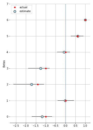
    pm.Multinomial('ll', n=1, p=p, observed = choice)

Hit the inference button, and you have the $\beta$ parameters recovered.

Final words

You can find the notebook here. The ones for the previous posts are up there as well. Next up the GEV model.