Logit Choice Model

I’ve been working my way through Kenneth Train’s “Discrete Choice Methods with Simulation” and playing around with the models and examples as I go. Kind of what I did with Mackay’s book. This post and the next have are some key takeaways with code from chapter 3 - Logit.

You can check out the notebooks for this post and the next here.

Utility model

A decision maker, $n$, faces $J$ alternatives. We can decompose the utility that the decision maker gets from each alternative as:

$V_{nj}$ is the known bit - what we can model and $\epsilon_{nj}$ is the iid error term.

Specifying $V_{nj}$

Linear. It does the job.

Also, as Train points out: “Under fairly general conditions, any function can be approximated arbitrarily closely by one that is linear in parameters.” You can get fancier though if you like and use something flexible like Cobb-Douglas if you like.

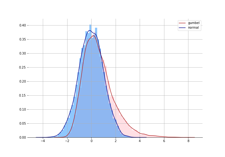
Gumbel errors

We get the logit model by assuming that that $\epsilon_{nj}$ follows a Gumbel distribution. Train claims this is not that hard a pill to swallow - it’s nearly the same as assuming the errors are independently normal. It just give fatter tails than a normal so allows the decision maker to get a little more wild.

But if we are comfortable with this assumption, then the difference of two Gumbel distributions:

follows as logistic distribution:

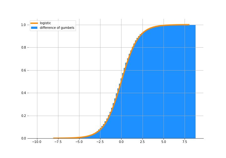
What might be harder tmo swallow is that the errors are iid. We are saying that the errors for a decision maker between alternatives are independent. Train doesn’t stress about this too much though; he claims that if you do a good job of specifying $V_{nj}$, then the rest is basically white noise.

But the key takeaway here is:

Violations of the logit assumptions seem to have less
effect when estimating average preferences that when
forecasting substitution patterns.* (pg. 36)

Nice. We’ll do an experiment later to test one of these violations as well.

From utility to probabilities

You can check out the book for the derivation. I’ll just outline the key bits that will be relevant when we do some simulations.

The probability that the decision maker chooses alternative $i$ over $j$ is:

A decision maker is simply comparing two utilities and picking the one that is higher. We don’t get to see those idiosyncratic errors but the decision maker experiences them.

Power and Limitations of the Logit

Logit has some nice properties - the bounds on $P_{ni}$, the sigmoid shape. And this has some implications on modelling which we won’t go into here.

The key thing here is to remember that the coefficients don’t have any meaning but their ratio does. So if you model utility as

Then the ratio of $\beta_1 / \beta_2$ has meaning. For example, if $x_1$ represents price and $x_2$ is operating cost, $\beta_1 / \beta_2$ represents the decision maker’s willingness to pay for operating cost reductions in up front price. Scale of the individual parameters doesn’t really matter - and this is also makes fitting them a little tricky sometimes.

Taste variation

Finally, some modelling.

Utility can be based on features of the car AND the household i.e we can model taste variation amongst the decision makers. Here’s the two param example from the book. Reminder that $n$ represents the decision maker and $j$ the alternative. Here ${PP}{j}$ is the purchase price for car $j$, and ${SR}{j}$ is the shoulder room in the car.

Each household has it’s own $\alpha$ and $\beta$ i.e. how much weight they put on these features of the car, based on some characteristics of the household - $M_n$ (size of family) and $I_n$ (income).

Substituting these into first equation:

So we are down to estimating $\rho$ and $\theta$. The rest of the $V_{nj}$ part of the utility are features of the car and household that are given.

We’re going to make up some data for households choosing between three cars. It’s similar to the example in the book but instead of 2 params ($\rho$ and $\theta$), let’s do 10 - because computers - and we’ll call them $\beta$s.

utility = (betas * households) @ cars.T + errors

choice = np.argmax(utility, axis=1)
car_choice_simple = np.zeros_like(utility)
car_choice_simple[np.arange(car_choice_simple.shape[0]), choice] = 1

That’s it. We’re done setting up the data. Now let’s see if we can recover the $\beta$ parameters (or rather, the ratios of these).

Outside option

We need to “pin down” one of the utilities else the model is not identified. Remember that scale of the betas doesn’t matter so an infinite sets of betas can fit the model. What we’ll do to get around this is to make the first car the “outside option” and say that the decision maker gets a utility of zero when she chooses that. The rest will be relative to this.

To achieve this, let’s make all the features relative to the first car.

cars_oo = cars - cars[0]

So now, all the features of car 1 are zeros which means the household will get a utility of zero as well.

Pymc3 model

The likelihood of the model is derived in section 3.7 of the book and is basically:

Look familiar? Yep, it’s a multinomial likelihood. You can write it out as a custom density, and I did, but the sampler is sooo much faster when using the optimized multinomial likelihood that comes built-in.

with pm.Model() as m_simple:

    betas_rest = pm.Normal('betas', 0, 1, shape=(1, n_params))

    utility_ = tt.dot((betas_rest * households), cars_oo[1:].T)
    utility_zero = pm.Deterministic('utility', tt.concatenate([tt.zeros((n_households, 1)), utility_], axis=1))
    p = pm.Deterministic('p', tt.nnet.softmax(utility_zero))

    pm.Multinomial('ll', n=1, p=p, observed = car_choice_simple)

How did we do?

trace = pm.sample(draws=500, model=m_simple, tune=5000, target_accept=0.95)

scaled_trace = trace['betas'].squeeze()
scaled_trace = scaled_trace / scaled_trace[:, 0].reshape(-1, 1)

That last line is “de-scaling” it. As we mentioned above, we’ll only look at the betas with reference to the first one.

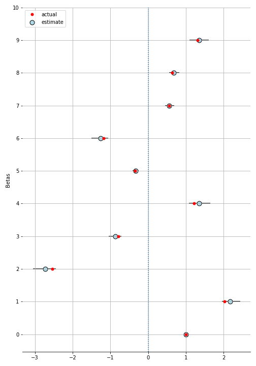
:D

You can dial up the gumbel noise and try to break it. I found it to be pretty robust.

When taste change randomly

Logit breaks down when tastes don’t vary systematically i.e. based on features of the household in our example, but rather each household has some randomness to their tastes. But as we’ll see and as Train points out, logit models are pretty robust to misspecification when you want to understand average tastes.

Now the household tastes have some randomness:

So the utility now becomes:

$\tilde{\epsilon}_{nj}$ is no longer iid since they are correlated within the same decision maker, $n$. Let’s simulate this data:

taste_errors = np.random.normal(4, 4, size = (n_households, n_params))
utility = (betas * households + taste_errors) @ cars.T + errors

We’ll skip the rest of the code here which is basically the same as above and go straight to the results.

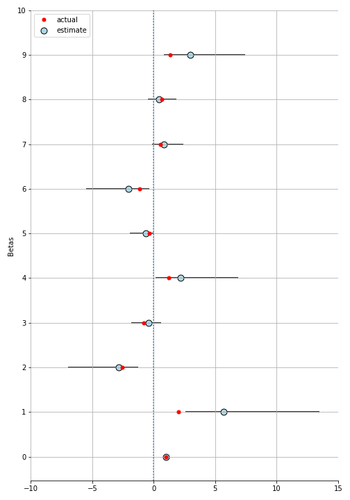
We get some large credible intervals but still not terrible. The actual value (mostly) lies within the 95% CI. In the notebook, I do another experiment where I model the taste errors as well it does a little better.

Substitution patterns

A feature (or bug if you’re not ok with the implications) of the logit model is how substitution occurs. It can be seen in two ways.

Independence from Irrelevant Alternatives (IIA)

For any two alternatives $i$ and $k$, the ratio of the logit probabilities is

No other alternatives but $k$, and $i$ enter this. So if some other alternative $l$ changes, it will effect the absolute probabilities of picking $k$ and $i$ but not the *ratio* of their probabilities.

Let’s check this out in our example (in logs to avoid overflow):

utility = (betas * households) @ cars.T + errors
p_base = sp.special.softmax(utility, axis=1)
p_base_ratio_12 = np.log(p_base[:, 1]) - np.log(p_base[:, 2])

# let's "improve" car 0
cars_0_improved = cars.copy()
cars_0_improved[0] = cars_0_improved[0] * 2

utility_car0_imp = (betas * households) @ cars_0_improved.T + errors
p_car0_imp = sp.special.softmax(utility_car0_imp, axis=1)
p_car0imp_diff12 = np.log(p_car0_imp[:, 1]) / np.log(p_car0_imp[:, 2])

np.all(np.isclose(p_car0imp_ratio_12, p_base_ratio_12))
#> True

This might not always make sense. The book provides the blue bus, red bus example. Say there are two modes of transport available - a blue bus and a car. Then a red bus gets introduced that travellers consider to be the same as the blue bus. The ratio of probabilities of blue bus and the car will clearly change. Half the people using the blue bus will switch to the red bus but none of the car drivers will. If you have this sort of situation, logit might not the right model.

Proportional Substitution

The same “issue” can be seen in terms of cross-elasticities. When an alternative improves, it changes the other probabilites proportional to their original values. It’s just easier to show you in code

diff_imp_car0 = p_car0_imp[:, 0] - p_base[:, 0]

# estimated change in car 1's probabilities as per proportion
diff_imp_car1_prop = diff_imp_car0 * p_base[:, 1]/(p_base[:, 1] + p_base[:, 2])

# actual change in car 1's probabilities
diff_imp_car1 = p_base[:, 1] - p_car0_imp[:, 1]

np.all(np.isclose(diff_imp_car1_prop, diff_imp_car1))
#> True

Next up - advantages of IIA

This post got a bit long so I’ll save the remainder for another (shorter) post. You can check that one out here. Notebooks for this post and the next are on github here.