In the last post, we talked about how this property of Independence from Irrelevant Alternatives (IIA) may not be realistic (see red bus / blue bus example). But, say you are comfortable with it and the proportional substitution that it implies, you get to use some nice tricks.
The first advantage is when the researcher only cares about a subset of alternatives. There are many ways to get to work - walk, bike, train, skateboard, skydive, helicopter etc. But if we only care about walk, bike, and train (and are ok with the IIA assumption) we can just select the people who chose these and drop all the other records. Neat.
The second one is that you can estimate model parameters, our $\beta$s from the last post, consistently on a subset of alternatives for each decision maker. In an experimental design, if there are 100 alternatives, the researcher can just provide a randomly selected set of 10 alternatives to each sampled decision maker. Or if you are using an existing dataset, model the decision maker’s choice set as the one they actually selected and nine other randomly chosen alternatives. You can see how this makes life easier.
Let’s demonstrate the second one with some fake data.
Estimation from a subset of alternatives
In this section I’ve shamelessly copied from Jim Savage’s (@jim_savage_) blog post. He did a great post on conjoint surveys and you don’t need a crappier python version of his post. I mainly ported his R/Stan code to Python/Pymc3 and added a few comments. You should check out his series of blog posts if you are interested in this topic.
Generate some data
Let’s make up some data
np.random.seed(23)

# # Number of attributes
P = 10
# Number of decision-makers
I = 1000
# Preferences
beta_true = np.random.normal(size=10)

# Number of choices per decisionmaker (between 5-10)
decisionmakers = pd.DataFrame({'i':np.arange(I),
                                'choices':np.random.choice(np.arange(5,11), I, replace = True)
                               })
Now we have a 1000 decision makers and each get a random number of alternatives between 5 and 10. Now let’s simulate each decision maker’s choice.
def make_choices(x):
    # Function that takes x (which contains a number of choices)
    # and returns some randomly conceived choice attributes as well
    # as a binary indicating which row was chosen

    X = np.random.choice([0,1], size=(x.choices.iloc[0], P))
    X = np.row_stack([np.zeros(P), X])
    u = X @ beta_true
    choice = np.random.multinomial(1, softmax(u))
    df = pd.DataFrame(X, columns = ['X_{}'.format(i) for i in range(P)])
    df['choice'] = choice

    return df

all_df = []
for dm, df in decisionmakers.groupby('i'):
    choice_df = make_choices(df)
    choice_df['i'] = dm
    all_df.append(choice_df)

decisionmakers_full = pd.concat(all_df, ignore_index=True)
So each decision maker has a binary matrix $X$ that determines the choices. Each row represents an alternative and columns if that alternative has that attribute or not. Then we multiply it through by the $\beta$s, how much decision makers value that attribute, to get the utility from each alternative. Softmax to convert to probabilities (see previous post on why you can do this) and generate choices using a multinomial.
We also add a row for the outside option that gives them zero utility - the X vector for that alternative is just a bunch of zeros.
Finally, let’s capture the indices for where each decision maker’s choice set starts and end.
indexes = decisionmakers_full.groupby('i').agg({'choice':{'start': lambda x: x.index[0], 'end':lambda x: x.index[-1]+1}})
indexes = indexes.droplevel(0, axis=1)
Fit the model
Let’s get the variables as numpy arrays and shared vars.
choice = decisionmakers_full['choice'].values
X = decisionmakers_full.filter(regex='X').values
N = X.shape[0]

start_idx = th.shared(indexes['start'].values)
end_idx = th.shared(indexes['end'].values)
And define the likelihood as a custom density in pymc3
class Logit(pm.distributions.distribution.Discrete):
    """
    Logit model

    Parameters
    ----------
    b : Beta params
    start : a list of start idx
    end : a list of end idx
    """

    def __init__(self, start, end, betas, *args, **kwargs):
        super(Logit, self).__init__(*args, **kwargs)
        self.start = tt.as_tensor_variable(start)
        self.end = tt.as_tensor_variable(end)
        self.betas = betas
        self.mode = 0.

    def get_dm_loglike(self, X, choice):

        def dm_like(s, e):
            s1 = tt.cast(s, 'int32')
            e1 = tt.cast(e, 'int32')

            p = tt.nnet.softmax(tt.dot(X[s1:e1], self.betas))
            return tt.dot(tt.log(p), choice[s1:e1]) + tt.dot(tt.log(1 - p), 1 - choice[s1:e1])

        likes, _ = th.scan(fn=dm_like,
                       sequences=[self.start, self.end])

        return likes

    def logp(self, X, choice):
        ll = self.get_dm_loglike(X, choice)
        return tt.sum(ll)
The rest is just putting it all together in a pymc3 model.
with pm.Model() as m:

    beta_ = pm.Normal('beta', 0, 4, shape=P)

    likelihood = Logit('likelihood', start_idx, end_idx, beta_, observed={'X':X, 'choice':choice})
    trace = pm.sample()
Results
Since scale doesn’t matter, we’ll scale $\beta_0$ to 1 and compare the other $beta$s relative to it.
scaled_trace = trace['beta'].squeeze()
scaled_trace = scaled_trace / scaled_trace[:, 0].reshape(-1, 1)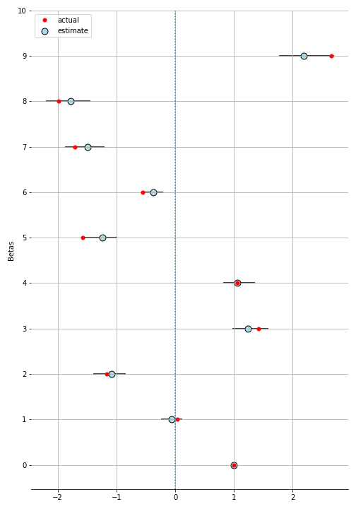
Voila! So the possible set of alternatives can be huge (in our case $2^p = 2^{10} = 1024$), but each decision maker only sees a small (5-10) number of alternatives with different features. We were able to take advantage of the IIA property and randomly select a subset of the alternatives to present to the decision maker.
You can find the notebook for this post here. The code here is not the most pythonic way of doing things. I just tried to keep it as similar to Jim’s code flow as possible so you can follow along with his posts but with the python code here. He also has a nice section on prior selection that I’m skipping here.