Poisson Density Estimation with Gaussian Processes

I have been slowly working my way through Efron & Hastie’s Computer Age Statistical Inference (CASI). Electronic copy is freely available and so far it has been a great though at time I get lost in the derivations.

In chapter 8, E&H show an example of a Poisson density estimation from a spatially truncated sample. Here, I implement the example using pymc3 and in addition to the latent linear model, I explore Gaussian Processes for the latent variable.

You can get the notebook from here.

The Problem

You can download the data from here. From CASI:

… shows galaxy counts from a small portion of the sky: 486 galaxies have had their redshift $r$ and apparent magnitude $m$ measured. Distance from earth is an increasing function of $r$, while apparent brightness is a decreasing function of $m$.

Note that this is truncated data. $r$ and $m$ are limited to

Here’s what the data table like:

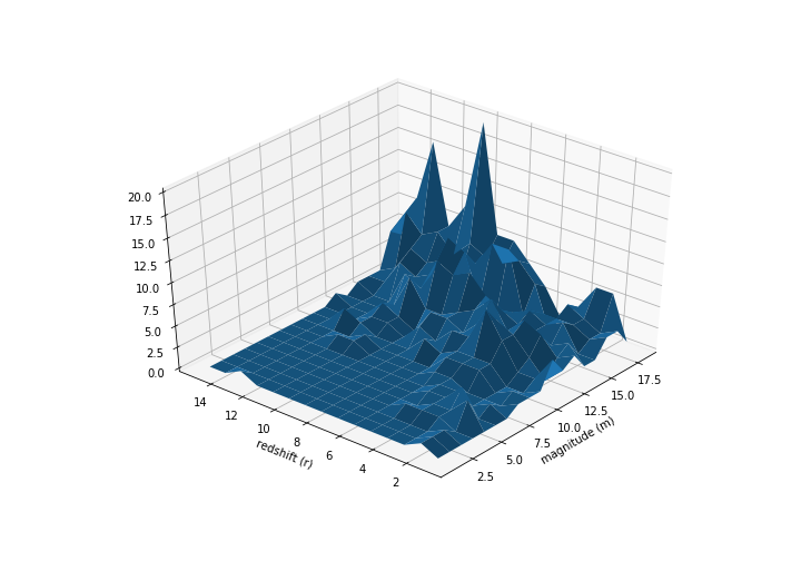
Our job is to fit a density to this truncated data. We are going to model this as

So each observation comes from a Poisson with a mean $\mu_i$. Actually, what we’ll model instead is $\lambda_i = \log(\mu_i)$.

Using Linear latent variable

The way Efron & Hastie model $\lambda$ is:

Where $\mathbf{X}$ is a “structure matrix” made up for features we crafted:

Where $\mathbf{r^2}$ is the vector whose components are the square of $\textbf{r}$’s etc. If we think that the true density is bivariate normal, then this makes sense. The log density of a bivariate normal is of this form.

Let’s setup this model in pymc3:

with pm.Model() as basic_model:

    alpha_0 = pm.Normal('alpha_0', 0, 10)
    alpha_1 = pm.Normal('alpha_1', 0, 10)
    alpha_2 = pm.Normal('alpha_2', 0, 10)
    alpha_3 = pm.Normal('alpha_3', 0, 10)
    alpha_4 = pm.Normal('alpha_4', 0, 10)
    alpha_5 = pm.Normal('alpha_5', 0, 10)

    latent = pm.Deterministic('latent', tt.dot(data_mat_n, tt.stack([alpha_0, alpha_1, alpha_2, alpha_3, alpha_4, alpha_5])))

    likelihood = pm.Poisson('like', tt.exp(latent), observed=data_long['val'].values)

Let’s see what our density looks like:

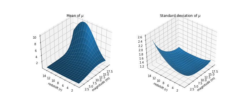
Because we setup a Bayesian GLM, not only do we have the mean values for $\mu$, we have the full distribution. The plot on the right shows the the standard deviation and as you might have expected, it’s high in the region where we didn’t have any data.

Using a Gaussian Process

If we are comfortable being agnostic of the functional form – and since I am not an astrophysicist, I’m quite comfortable – we can use a 2-d gaussian process. You may want to out the previous posts on Gaussian Processes:

1. Intro to gaussian processes
2. Latent GP and binomial likelihood

So now our lambda is:

Here $x$ is $(r, m)$, a point on the grid and $f(x)$ is a Gaussian Process:

(Sorry about the loose notation).

Here’s the model in pymc3:

with pm.Model() as gp_model:

    ro = pm.Exponential('ro', 1)
    eta = pm.Exponential('eta', 1)

    K = eta**2 + pm.gp.cov.ExpQuad(2, ro)
    gp = pm.gp.Latent(cov_func=K)

    # Note that we are just using the first two columns of
    # data_mat which correspond to 'r' and 'm'
    latent = gp.prior('latent', X=data_mat[:,:2])

    likelihood = pm.Poisson('like', tt.exp(latent), observed=data_long['val'].values)

And the resulting density:

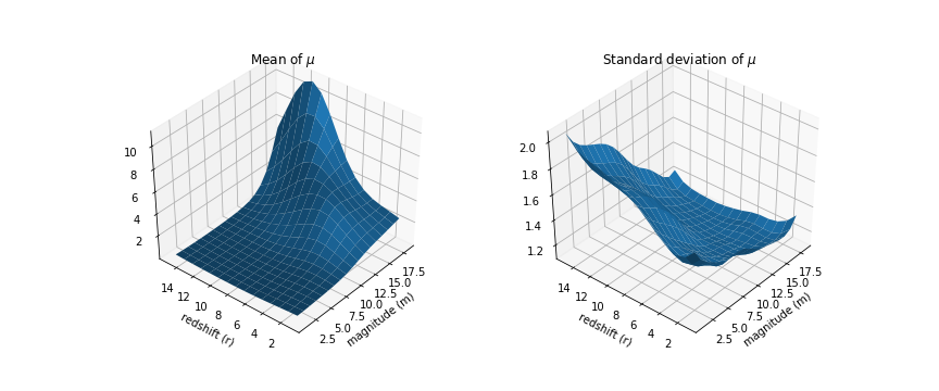
The standard deviation surface looks a lot bumpier but the general trend is similar; it is higher in areas where we have little data. Very cool, but is that model any good?

Deviance residual

Efron & Hastie use the deviance residual to check the goodness of fit.

Side note: this is based on KL-divergence so I couldn’t figure out how they got around the problem of 0. For KL-divergence you need to have non-zero probabilities in the entire domain. I just ignore the ‘NaNs’ resulting from it and pretend like nothing happened.

def deviance_resid(y, mu):
    def D(mu1, mu2):
        return  2 * mu1 * (((mu2/mu1) - 1) - np.log(mu2/mu1))

    return np.sign(y - mu) * np.sqrt(D(y, mu))

Comparing the sum of squares of the residual, we get 109.7 for the GP model and 134.1 for the linear model. This next plot shows these residuals.

Looks like the GP model fits the top left corner better than the linear model but it also fits that stray bottom right dot that makes me worry that it might be overfitting. One way around it would be to use a different implementation of GP that allows for additive noise.

We can check for overfitting by looking at WAIC for the two using pymc3’s compareplot:

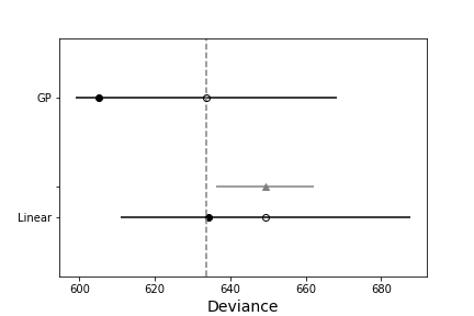
Looks like the GP-model is the better model. Check out the notebook and let me know if there are ways you would improve this. How can we implement this using gp.marginal or gp.conditional so that we can include additive noise?