[Survival models] Cox proportional hazard model

In the previous blogpost, we talked about the hazard function - the probability that the event happens at time $t$ given that you it hasn’t till time $t$. In the Cox proportional hazard model, we assume the hazard function is:

Some interesting things to point out here:

• time $t$ only occurs in $h_0(t)$
• covariates, $x_i$ only occur in the $exp$ bit

So there is some base hazard rate $h_0(t)$ and the only way it varies for units with different characteristics is through the $exp$ bit. So why is it called “proportional” hazard model?

Imagine a simple model where:

And we have a unit $i$ with $x_{i1} = z$ and another unit $j$ with $x_{ji} = a \cdot z$ so let’s see the hazard for each:

And

So the hazard ratio of the two is:

So no matter what the $t$ is, the hazard ration between these two is always some constant. Another way is to note that:

where $c = exp(b_1 (a -1 )z)$. So $h_i(t)$ is proportional to $h_j(t)$ - times does not make an appearance in the coefficient. This assumption may not be true and there are a bunch of tests you can do to check it.

Alright. Enough with the theory.

Partial likelihood

I’m not going to derive it. The internet is your friend.

where $R_j$ is the risk set - people at risk of death/event when the event for $j$ occurs. This should look familiar - it’s softmax. The intuition follows from there. So we want to pick the betas that maximise the likelihood of the event happening out of all the units at risk.

Log-likelihood just needs some $algebra$:

Now all we need to code it up with jax for some sweet sweet autograd.

Minimize negative log likelihood

import jax.scipy as jsp
import jax

@jax.jit
def neglogp(betas, riskset=riskset, observed=observed):
    betas_x = betas @ x.T
    riskset_beta = betas_x * riskset
    ll_matrix = (betas_x - jsp.special.logsumexp(riskset_beta, b=riskset, axis=1))
    return -(observed * ll_matrix).sum()

If you know numpy and scipy, you know a lot of jax.

P.S: Took me forever to realise that logsumexp take a weight argument as b. No idea why statsmodels doesn’t use this.

Ok. Now all we need is to minimize it. Here comes the magic of autograd

from jax import grad, hessian
from scipy.optimize import minimize

dlike = grad(neglogp)
dlike2 = hessian(neglogp)
res = minimize(neglogp, np.ones(2), method='Newton-CG', jac=dlike, hess=dlike2)
res.x

>>> DeviceArray([-0.14952305, -0.16527627], dtype=float32)

You can compare this to statsmodels or lifelines package. It’s in the notebook - you can check it out.

Let’s get Bayesian

Blackjax is a pretty sweet package with a lot of sampling methods. Let’s use the NUTS sampler (yes - i know, that’s calling it a “sampler sampler”). Let’s use it to get some samples. This is basically the example in the blackjax documentation.

First we need the posterior probability which is simply the prior $\times$ the likelihood. In log terms:

def logprior(betas):
    return jsp.stats.norm.logpdf(betas, 0, 1.0).sum()

logprob = lambda x: logprior(**x) + neglogp3(**x)

Ok. Let’s setup the initial values and the kernel.

initial_position = {"betas": jnp.ones(2)}
initial_state = nuts.new_state(initial_position, logprob)

inv_mass_matrix = np.array([0.5, 0.5])
step_size = 1e-3

nuts_kernel = jax.jit(nuts.kernel(logprob, step_size, inv_mass_matrix))

and the inference loop for samples:

def inference_loop(rng_key, kernel, initial_state, num_samples):
    def one_step(state, rng_key):
        state, _ = kernel(rng_key, state)
        return state, state

    keys = jax.random.split(rng_key, num_samples)
    _, states = jax.lax.scan(one_step, initial_state, keys)

    return states

    rng_key = jax.random.PRNGKey(0)
    states = inference_loop(rng_key, nuts_kernel, initial_state, 1000)

    beta_samples = states.position["betas"].block_until_ready()

Now let’s get some samples:

rng_key = jax.random.PRNGKey(0)
states = inference_loop(rng_key, nuts_kernel, initial_state, 1000)

beta_samples = states.position["betas"].block_until_ready()

Here’s the trace from it:

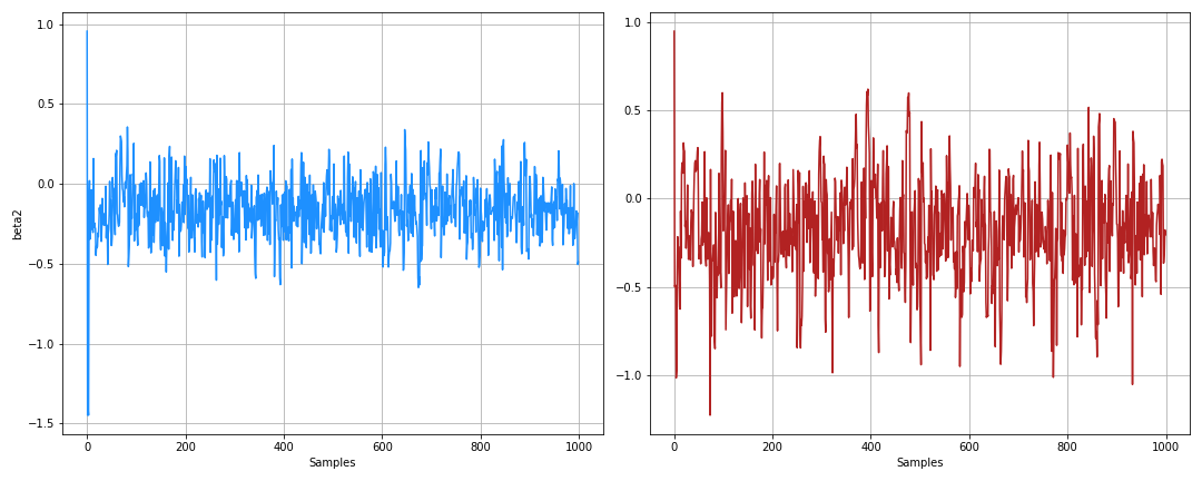
And the posterior:

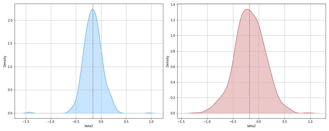
And there you have it folks - some nice confidence intervals.

Final words

Ok - I cheated a little bit. I removed ties in the database. If you have ties you need a slight change to the likelihood - check out the statsmodels code for efron_loglike or breslow_loglike.

The point of this was also to play around with jax and blackjax. Mission accomplished. Let’s look at some parametric models next time around.