[Survival models] Censored data and intro to survival models

I recently gave a short intro to survival models to the team as part of a knowledge share session. The goal was to motivate why we should care about censored models.

Discussion on censoring

Data Setup

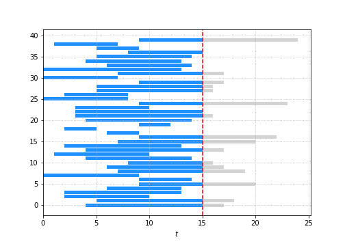
You are given a dataset with kids enrolled in school. Some have dropped out and some haven’t.

mean_time = 10
n_samples = 40
lifespan = np.random.poisson(mean_time, size=n_samples)
start_time = np.random.randint(0, 10, size=n_samples)

Let’s calculate the sample average.

end_time = start_time + lifespan
print("Empirical mean lifespan is: ", np.mean(lifespan))

>>> Empirical mean lifespan is:  9.35

That fairly close to 10.

But kids started at different times and we don’t see all of them dropping out. We only observe the ones that have dropped out till today.

Say today is $t = 15$ then you don’t get to see all the events that happen after $t = 15$ i.e. the bits in grey.

censored data

So here’s the question:

What is the average “lifespan” of the student population?

Take 1: Just take the mean of the observed values

Ok. Using the clipped times naively:

clipped_lifespans = clipped_end_times - start_time
np.mean(clipped_lifespans)

>>> 7.975

That’s quite off the true value of 10 or even the sample mean of 9.35. Why this doesn’t work is obvious here; we have bias samples. We are assuming that the students that dropped out in the future, dropped out right now. Oof.

Take 2: Only use those that are not censored

lifespan[end_time < 15].mean()

>>> 7.545454545454546

That doesn’t work either. Why is a bit more interesting. It’s related to the inspection paradox. Imagine that all students started on the same day. By excluding the censored one, we are dropping the samples that go for longer –> bias.

MLE estimation

Given parameters $\Theta$ (in our case it is just the $\lambda$ of the Poisson distribution), likelihood is made up of two parts:

For uncensored data: Probability of observing this data point - that’s $f(x_i \theta)$
For censored data: Probability of observing that this data point hasn’t occurred yet - that’s $F(x_i \theta)$

Where $f(x)$ is the pdf and $F(x)$ is the cdf. Dropping the conditional on $\Theta$ for brevity:

\[\begin{aligned} \mathbb{L\left(\theta\right)} &= \prod_{d \in D} f(x_d) \prod_{r \in R} (1 - F(x_d))\\ ll\left(\theta\right) &= log \left(\prod_{d \in D} f(x_d) \prod_{r \in R} (1 - F(x_d))\right)\\ ll\left(\theta\right) &= \sum_{d \in D} log(f(x_d)) + \sum_{r \in R} log(1 - F(x_d))\\ \end{aligned}\]

Let’s code this up in jax so we can get some gradients for free.

import jax.numpy as jnp
import jax.scipy.stats as jst

is_clipped = (end_time > 15)

def negloglikelihood(log_lambd):

    censored = jnp.log1p(-jst.poisson.cdf(clipped_lifespans[is_clipped],
                                          jnp.exp(log_lambd))).sum()
    uncensored = jst.poisson.logpmf(clipped_lifespans[~is_clipped],
                                    jnp.exp(log_lambd)).sum()

    return -(uncensored + censored)

Some questions for you here (that I won’t answer):

Why the use log lambda only to take exp later?
What is log1p?

And let’s get the gradient.

from jax import grad
dlike = grad(negloglikelihood)

Man I love autograd. Makes me a worse mathematician but a much better data scientist.

Then we can use our vanilla gradient descent

log_lambd = 1.0
log_lambd_new = 1.0

for i in range(30):
    dx = dlike(log_lambd)
    log_lambd_new -= dx * 0.001

    if (np.abs(log_lambd_new - log_lambd) < 0.0001):
        break
    else:
        log_lambd = log_lambd_new

np.exp(log_lambd)

>>> 9.312129

or we can use scipy’s optimiser:

from scipy.optimize import minimize
res = minimize(negloglikelihood, 1.0, method='BFGS', jac=dlike)
np.exp(res.x[0])

>>> 9.314376480571012

Hey! Look ma - parameter recovered.

Let’s connect this to some survival analysis concepts.

Survival model concepts

Survival function

The probability that the event has not occurred till t (so occurs somewhere in the future)

\[S(t) = Pr(T > t)\\ S(t) = 1 - Pr(T < t)\\ S(t) = 1 - F_T(t)\\\]

Hazard function

Given that the event has not occurred till now, what is the probability that it occurs at time t

\[\begin{aligned} h(t) &= \lim_{\delta t \rightarrow 0 } \; \frac{Pr( t \le T \le t + \delta t | T > t)}{\delta t}\\ h(t) &= \frac{-S'(t)}{S(t)} \end{aligned}\]

and solving this gives us:

\[S(t) = \exp\left( -\int_0^t h(z) \mathrm{d}z \right)\\ S(t) = \exp\left(-H(t) \right)\]

where $H(t)$ is the cumulative hazard function. The cumulative hazard function is a mind fuck - maybe one way to think about it is the number of times a person would have died till time $t$. Assuming they are brought back to life each time. Even though we know they only have one life. Anyway… moving on.

I love this diagram from the lifelines package:

surv_funcs map

Kaplan-Meier charts

At each time period, we can non-parametrically calculate the survival function:

\[\hat{S}(t) = \prod_{t_i \lt t} \frac{n_i - d_i}{n_i}\]

where:

$n_i$ is the number exposed; and
$d_i$ is the number of events or “deaths”

So of the people who were exposed, what proportion of them survived. How does censored data work into this? Note that $n_i$ contains uncensored peeps but the censored ones only make it into the numerator.

Let’s use some data from Ibrahim et al:

import pandas as pd

cancer = pd.read_fwf("./e1684.jasa.dat").drop(0)
cancer = cancer.loc[cancer.sex != "."]
cancer['sex'] = cancer.sex.astype(int)
cancer["observed"] = (cancer["survcens"] == 2)

And let’s use the lifelines package to check out the survival curve - since we get confidence intervals with it.

from lifelines import KaplanMeierFitter
kmf = KaplanMeierFitter()

T = cancer["survtime"]
E = cancer["observed"]

plt.subplots(figsize=(7, 5))
kmf.plot_survival_function();
plt.grid(ls=":")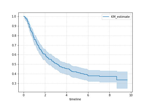

censored data

Conclusion

Ok - I’m going to stop here. That’s enough of an intro. Next time: cox proportional models and parametric models. If I ever get the time.