Large-Scale Hypothesis Testing (Part 2)

In part 1, we looked at Empirical Bayes Large-Scale Testing where we defined the data generating process as a mixture model. In this post, instead of empirically estimating $S(z)$, we assume it’s a mixture of two gaussian and define a mixture model in pymc3. We finish by considering the local false discovery rate, which has a much cleaner bayesian interpretation.

This post is also based on Chapter 15 of Computer Age Statistical Inference (CASI) by Bradley and Efron.

Large Scale Testing as a mixture of gaussians

In the previous post, we defined our data generating process for the z-scores of the gene activity t-tests as:

Where $S_0(z)$ and $S_1(z)$ are the survival function of the null distribution (the standard normal), and the non-null distribution, respectively. We showed the error rate to be:

Problem as a mixture of normals

Instead of estimating $S(z)$ using the empirical distribution, we assume $S_1(z)$ is also a normal and just model it as a mixture. Here’s the model in pymc3:

with pm.Model() as m:

    sd = pm.HalfNormal('sd', 3)

    dist1 = pm.Normal.dist(0, 1)
    dist2 = pm.Normal.dist(0, sd)

    pi = pm.Dirichlet('w', a= np.array([0.9, 0.1]))
    like = pm.Mixture('like', w=pi, comp_dists=[dist1, dist2], observed=x1)

Here are the posterior draws:

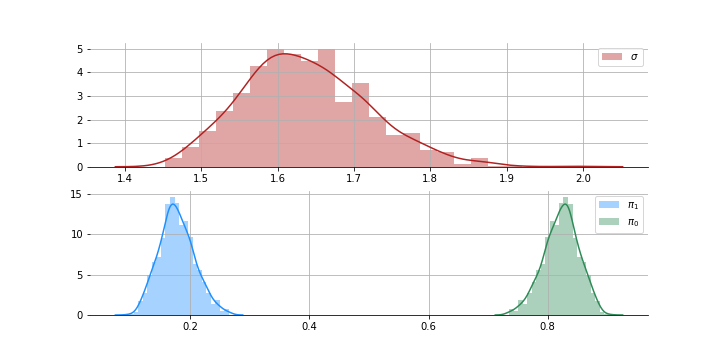
The posterior for sd is mostly between 1.5 and 1.8 which makes sense. Now that we have $S_1$ and $\pi_0$ we can calculate the distribution of $S(z)$. Plug these into the $Fdr$ equation above and we can identify the non-nulls with some error rate $q$.

F1 = st.norm(0, sample['sd']).cdf(x1.reshape(-1, 1))
F0 = st.norm(0, 1).cdf(x1.reshape(-1, 1))

S = (sample['w'][:, 0] * (1 - F0)) + (sample['w'][:, 1] * (1 - F1))
S_ratio = (1 - F0) / S

low, high = np.percentile(S_ratio, [2.5, 97.5], axis = 1)

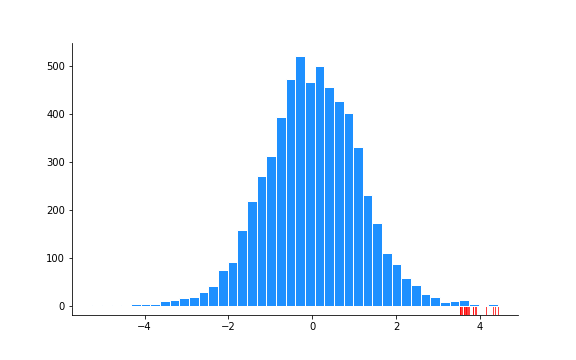
significant_idx = np.argwhere((high <= 0.1)).squeeze()

Here’s the histogram of the 6033 $z$ values again with the significant results show in the rug plot:

You could repeat this and use the cdf instead of the survival functions in the code above to get the negative significant values.

Local False-Discovery Rates

After this whole Bayesian re-interpretation, it doesn’t really make a lot of sense to be looking at tail-area, $z_i \geq z_0$. Why not just look at the probability or pdf of $z_i = z_0$. What we want is the local false discovery rate (fdr):

A similar logic follows to the tail-area false discovery rate and you can check out the book for more details. But you may not be too surprised to learn that we get something very similar to the tail area fdr:

Fitting $f(z)$

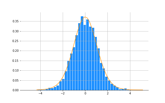
We could estimate $\hat{S}(z_0)$ empirically and it was fairly smooth since we were working with a cdf. Using the same method here would give us a noisy estimate since we’ll only have a point or two to estimate a pdf, $f$. We need to smooth it out. You could do this in a number of ways but CASI chooses to fit a Poisson distribution to the binned values with the latent variable modelled as a 4th degree polynomial, so let’s go with that.

from sklearn.preprocessing import PolynomialFeatures
import statsmodels.api as sm

vals, edges = np.histogram(-trans_t, bins=45, density=True)
mid_points = (edges[0:-1] + edges[1:]) / 2

X = PolynomialFeatures(degree=4).fit_transform(mid_points.reshape(-1, 1))
y = vals

m = sm.GLM(y, X, family=sm.families.Poisson(), ).fit()
y_hat = m.predict()

And here’s the fit:

Calculate fdr

We know that $f_0(z)$ is a standard normal and now have a fitted $f(z)$. We just need to plug this back into the equation for fdr (we can assume $\pi_0$ to be close to 1). These two functions can do that for us:

def fhat(z, m):
    n_dims = m.params.shape[0]
    poly_vals = PolynomialFeatures(degree=(n_dims - 1)).fit_transform(z.reshape(-1, 1))

    return np.exp(poly_vals.squeeze() @ m.params)

def fdr_hat(z, m, pi0 = 0.9):
    return pi0 * st.norm.pdf(z) / fhat(z, m)

Now we can plot the local false discovery rates and the tail-area false discovery rates to do a comparison:

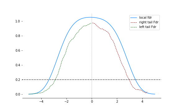
The local fdr is a lot stricter. In both tails, it requires a larger threshold for the same rate of false discovery $q$, shown in the figure at 0.2.

Full bayesian model again

Earlier in the post, we fitted a mixture model. We can use that here again. $f_1(z)$ is a zero-mean normal with standard deviation between 1.5 and 1.8. We can calculate the local fdr as before using this.

Let’s add this to the plot above:

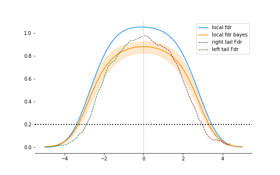
The bayesian version is not as conservative as the glm fitted local fdr but results are pretty similar. And hey! Confidence intervals.

Conclusions

You probably been Bonferroni-ing it like me. And that’s perfecting fine in most cases where you are testing 5-10 hypothesis. When you start getting in the thousands, you can actually do much better. You can use the other estimates to inform the significance of a particular estimate, a property you usually associated with bayesian methods. And there is indeed a bayesian interpretation.

The notebook can be found here. I stopped cleaning up notebooks at some stage. It has a lot of failed experiments and other extensions but it’s messy and badly commented. Don’t judge me.

Thanks for reading. Happy hunting.