Large-Scale Hypothesis Testing (Part 1)

We take a short detour from Bayesian methods to talk about large-scale hypothesis testing. You all are probably quite familiar with the p-hacking controversy and the dangers of multiple testing. This post isn’t about that. What if you are not confirming a single hypothesis but want to find a few interesting “statistically significant” estimates in your data to direct your research?

This post is based on Chapter 15 of Computer Age Statistical Inference (CASI) by Bradley and Efron.

Large-scale Testing

The example in CASI is of microarray study of 52 prostate cancer patients and 50 controls. This microarray allows you to measure the individual activity of 6033 genes. We want to identify which of the difference in gene activity between the patients and the controls is significant. In hypothesis testing land, that’s 6033 t-tests.

The null Hypothesis

If we have $i$ genes, we have $i$ hypothesis tests and therefore $i$ nulls. Our null hypothesis, $H_{0i}$ is that patients’ and the controls’ responses come from the same normal distribution of gene $i$ expression. The t-test for gene $i$ will follows a Student $t$ distribution with 100 (50 + 52 - 2) degrees of freedom. Let’s map this to the normal distribution:

where $F_{100}(t_i)$ is the cdf of the $t_{100}$ distribution and $\Phi^{-1}$ is the inverse cdf of the normal distribution.

Now we can state our null hypotheses as:

You probably already know that you can’t just run all the 6033 hypothesis tests and pick the ones with p < 0.05. 5% of them will be “significant” even when the null is true. Even if you don’t remember the definition of p-value from school, you can just simulate it to prove it to yourself:

# Simulation 100 t-tests with 0.05
dist1 = np.random.normal(0, 1, size = (1100, 100))
dist2 = np.random.normal(0, 1, size = (1100, 100))

_ , p_vals = st.ttest_ind(dist1, dist2, axis = 1)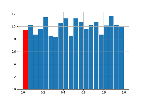

The red bar shows the 5% of the samples that show up as significant at the 5% level even though we know that both samples came from the same distribution.

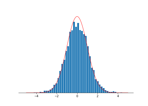
For the prostate data, the z-vals match the null distribution quite well. Maybe it’s a little fatter on the tails suggesting we may have some interesting stuff going on.

Bonferroni bounds

You probably also remember the Bonferroni correction. If you’re going to do 6033 hypothesis tests then the one-sided Bonferroni threshold for significance is $\alpha / 6033$. The idea is to keep the family-wise error rate, the probability of making even one false rejection, to below $\alpha$.

Using the prostate data, 4 genes that shows up as significant at the Bonferroni threshold of $\frac{0.05}{6033} = 8.3 \times 10^6$.

Holm’s procedure

Holm’s is bit better than Bonferroni. Here’s how that goes:

1. Sort p-vals from smallest to largest:

   \[p_{1} \leq p_{2} \leq ... \leq p_{i} \leq ... \leq p_{N}\]

2. Let $i_0$ be the smallest index $i$ such that

   \[p_{i} > \alpha / (N - i + 1)\]

3. Reject all the $H_{0i}$ for $i < i_0$.

On the prostate data this gives 5 significant genes, one more than the Bonferroni correction.

Benjamini–Hochberg FDR Control

Most of the time when we’re doing this sort of multiple testing, we’re going on a fishing expedition. We are hoping that to find some interesting things worth further investigating. It’s more exploratory analysis than inference. So another way we may think about the problem is that we want to minimise the probability of making an error - rejecting the null when we shouldn’t have.

Here’s a figure taken from CASI:

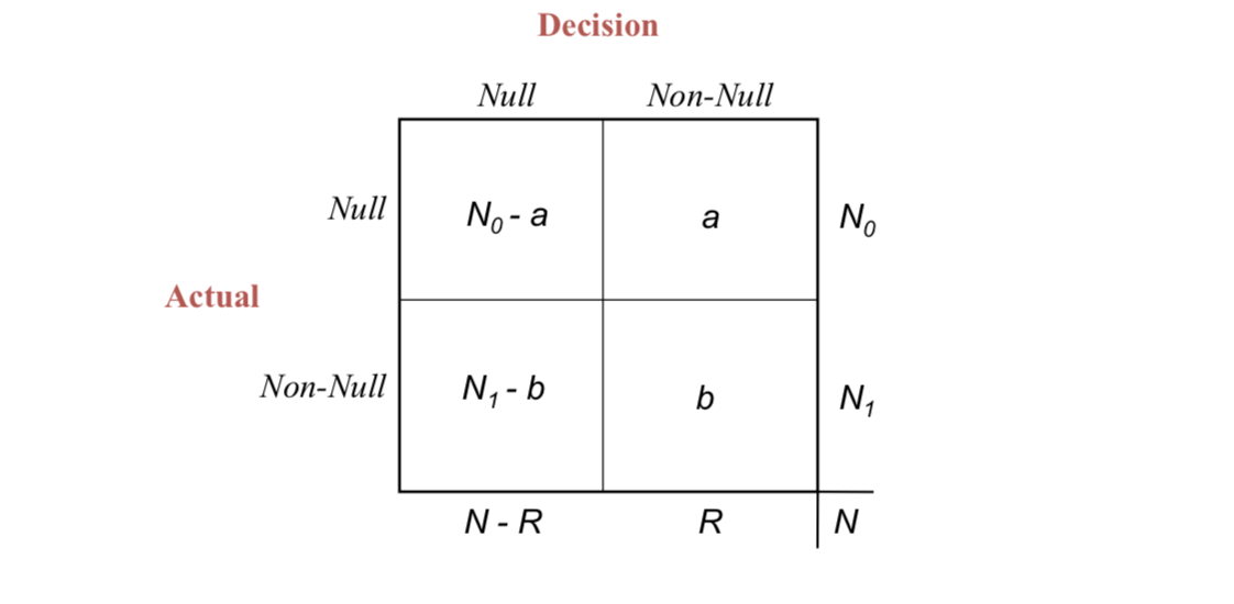
Under some decision rule, $\mathcal{D}$, you choose to reject $R$. $a$ of them would be wrong (should not be rejecting) and $b$ would be correct. We don’t know $a$, so we can’t calculate the “false-discovery proportion” (Fdp) of $\alpha / R$. But under certain circumstances we can control its expectation:

We’d want to come up with a decision $\mathcal{D}_q$ that keep this $FDR$ below $q$:

Here’s the procedure that does that. See book for theorem and proof.

1. Sort p-vals from smallest to largest:

   \[p_{1} \leq p_{2} \leq ... \leq p_{i} \leq ... \leq p_{N}\]

2. Define $i_{max}$ to be largest index for which

   \[p_{i} \leq \frac{i}{N}q\]

3. Reject all the $H_{0i}$ for $i < i_{max}$.

Comparison with Holm’s

Holm’s rejects null, $H_{0i}$, if:

and $\mathcal{D}_q$ has threshold:

For the prostate data, we can compare the two methods:

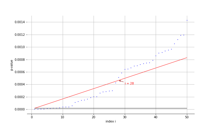
FDR is a lot more generous and rejects the 28 most extreme z-vals. The slope for the Holm’s procedure is barely noticeable.

Empirical Bayes Large-Scale Testing

Ok - I lied. The thing that really got me writing this blogpost was restating the multiple testing problem in a Bayesian framework. The algorithm for $\mathcal{D}_q$ above can be derived from this Bayesian re-interpretation.

Let’s think about it as a generative model. Each of the $N$ cases (6033 in the prostate example) is either null or not-null. So the $z$-score we came up with above come from either the null distribution $f_0(z)$ or some other, non-null distribution, $f_1(z)$. Let’s say the probability of a null is $\pi_0$ and and non-null is $\pi_1 = 1 - \pi_0$. So we have:

In the prostate case, $\pi_0$ is close to one; most of the genes differences are not significant. And $f_0$ is the standard normal here (though it doesn’t always have to be). Few other definitions: $F_0$ and $F_1$ are the cdfs for $f_0$ and $f_1$ with “survival curves”:

What we actually observe is a mixture of the two. So we have:

Now let’s define the Bayesian Fdr as the probability that the case really is null when our $z$ value is greater than some rejection threshold, $z_0$:

We know that $\pi_0$ is close to one. We also know that our null distribution is a standard normal so $S_0(z_0)$ is just $1 - \Phi(z_0)$. Only thing left is to figure out $S(z_0)$ and we just do this empirically:

So we now have the empirical false discovery rate:

Equivalence to Benjamini-Hochberg

Now here’s the fun bit. Note that the p-value for $i$ is the probability that you observe something this or more extreme given the null hypothesis. That’s exactly what $S_0(z_i)$ is. So we have:

and $\hat{S}(z_i) = i / N$ if $z_i$ are sorted and $i$ is the index. Sub these into the equation in step 2 above and you get:

the last line is by multiplying $\pi_0$ on both sides.

Final words

So when you are using the Benjamini-Hochberg algorithm, you are rejecting the cases where the posterior of coming from the null distribution is too small.

There are other things to talk about. With the Bayesian framework, why look at $ Pr(\text{case i is null} \vert z_i > z0)$ when we can do $Pr(\text{case i is null} \vert z_i = z0)$. It makes a lot more sense. These lead us to local false-discovery rates and another blog post.

The untidy notebook can be found here. Thanks for reading.