Jackknife, Non-parametric and Parametric Bootstrap

In frequentist statistics, you want to know how seriously you should take your estimates. That’s easy if you’re doing something straight forward like averaging:

or OLS¹:

If you want to get any fancier, chances are you don’t have a nice formula for it.

Say we observe an iid sample $\boldsymbol{x} = (x_1, x_2, … , x_n)’$ from some probability distribution $F$:

And we want to calculate some real valued statistic $\hat{\theta}$ that we get by applying some algorithm $s(\cdot)$ to $\boldsymbol{x}$,

and want to get a standard error for our $\hat{\theta}$. The jackknife and the bootstrap are two extremely useful techniques that can help. In the post, I’ll go through these and the parametric version of the bootstrap using a bunch of examples.

Most of this post is built around Chapter 10 of Computer Age Statistic Inference by Efron and Hastie. You can get the book freely online here. You can get the notebook for all the code here.

The Jackknife

Let $\boldsymbol{x}_{(i)}$ be the sample with $i^{th}$ element $x_i$ removed. Now your jacknife estimate of the standard error is:

Let’s summarise what we are doing here. If we have $n$ samples,

1. We calculate the statistic, $\hat{\theta}$, $n$ times, with one of the sample values left out each time.
2. We take the average of these $n$ statistics and get ($\hat{\theta}_{(\cdot)}$)
3. Plug it in to (1) and you’re done.

The good stuff

It’s nonparamteric - we made no assumptions about the underlying distribution $F$. It’s automatic - If you have $s(\cdot)$, you can get your $\hat{se}_{jack}$.

The bad stuff

Assumes smooth behaviour across samples: Samples that are different by one $x_i$ should not have vasty different estimates. Check out the book (pg. 157) for similarities with Taylor series methods, and therefore, it’s dependence on local derivatives. We’ll see an example with lowess curves where this is violated.

The Nonparametric Bootstrap

The ideal way to get standard errors would be to get new samples from $F$ and compute your statistic. But $F$ is usually not known. Bootstrap uses the estimate $\hat{F}$ instead of $F$.

Algorithm is quite simple. You take a bootstrap sample:

where $x_i^* $ is drawn randomly with equal probability and with replacement from $(x_1, x_2,…,x_n)$.

Take this bootstrap sample, $\boldsymbol{x}^* $ and plug it into your estimator and get an estimate:

Do this $B$ times where $B$ is some large number to get an estimate for each bootstrap sample.

Calculate the empirical standard deviation of the $\hat{\theta}^{* b}$ values:

To summarise:

1. Get $B$ samples with replacement of size $n$ from $(x_1, x_2,…,x_n)$.
2. Calculate your statistic, $\hat{\theta}$, for each of these samples.
3. Take the empirical standard deviation of all these $\hat{\theta}$s to get your standard error.

The good stuff

Like the jackknife, it’s completely automatic. It’s more dependable than jackknife for non-smooth statistics since it doesn’t depend on local derivatives.

The bad stuff

Computationally, it can be quite expensive.

Example 1: standard errors for lowess

I’m going to skip the code for the jackknife and bootstrap here since it’s fairly straightforward (you can checkout the notebook if you like) and skip to the results:

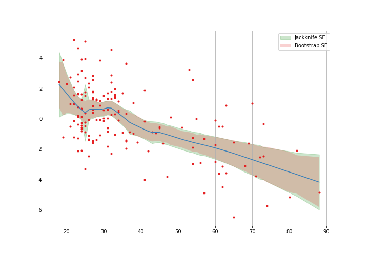
Note that they are pretty similar most of the way but the jackknife estimates get funky around 25. In Efron and Hastie’s words: “local derivatives greatly overstate the sensitivity of the lowess curve to global changes in the sample $\boldsymbol{x}$”

Example 2: The “eigenratio”

We have a table of results of 22 students taking 5 tests. The pairwise correlations of these scores is:

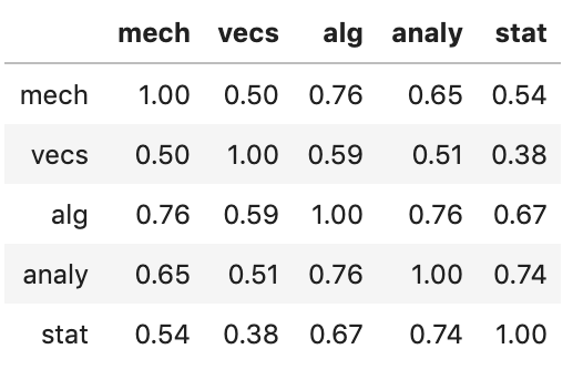
We want to the calculate the standard errors for the “eigenratio” statistic for this table:

which says how closely the five scores can be predicted by a single linear combination of the columns. The plot below shows the bootstrap results:

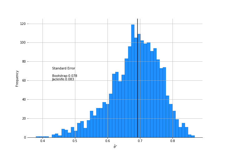
Few interesting things to note here. The jackknife estimate of standard error is larger than the bootstrap’s. The distribution isn’t normal. If you decided to get a confidence interval using +/- 1.96 $\hat{se}$ for a 95% coverage, you’d be quite biased.

The Parametric Bootstrap

I like parametric methods. Often there are distributional assumptions you are willing to make that help your model along substantially. If I asked you what is the effect on sales as if you increase the discount, you’d be comfortable saying it’s some monotonically increasing function. That’s information that you can’t include in your random forest model (easily).

The same applies here. If you are comfortable assuming your samples come from some distribution, you can just sample from that distribution to get your bootstrap samples.

For example, if your sample $\boldsymbol{x} = (x_1, x_2, …, x_n)$ comes from a normal distribution:

then $\hat{\mu} = \bar{x}$, and a parametric bootstrap sample is $\boldsymbol{x}^* = (x_1^* , x_2^* , …, x_n^* )$. The rest of it proceeds as normal.

Example: Glomerular filtration rates (gfr)

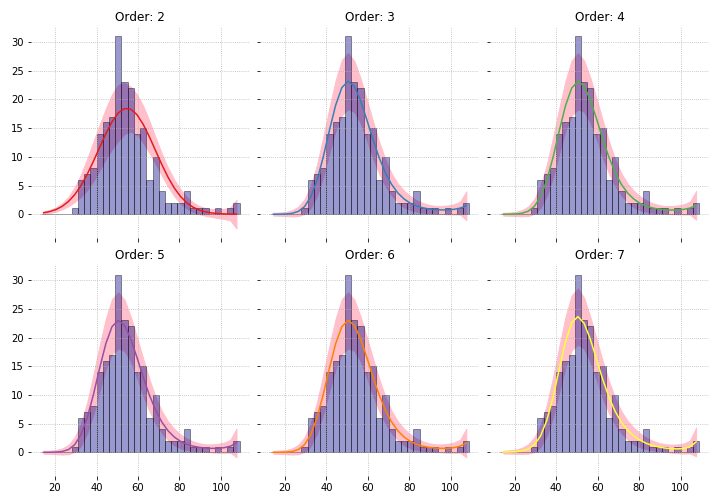
We have binned gfr data from 211 kidney patients. Say we are comfortable claiming that this comes from a Poisson distribution and have fitted a parametric model. The figure below shows models fitted with different order of polynomials.

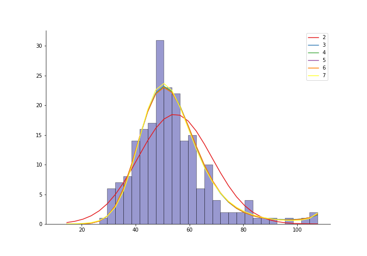
How accurate are these curves? We can use parametric bootstrapping to get their standard errors.

First, let’s create the higher order variables.

deg_freedom = 7

for d in range(2, deg_freedom+1):
    df["xs"+str(d)] = xs**d

Now let’s do some bootstrapping for each of the fits:

endog = df.y.values               # the bin counts
exog_cols = ['xs', 'intercept']   # the bin centre value is xs
models = []
lnk = sm.families.links
all_fitted_vals = {}
for d in range(2, deg_freedom + 1):
    exog_cols.append('xs'+str(d))

    # fit the model
    model = sm.GLM(endog=df.y.values, exog=df[exog_cols].values,
      family=sm.families.Poisson()).fit()

    # Generate samples from fitted model
    samples = np.random.poisson(model.fittedvalues,
                                size=(200, len(df)))

    # For each sample, run the 'statistic' i.e. the fit again
    fitted_vals = []
    for sample in samples:
        sample_model = sm.GLM(endog=sample, exog=df[exog_cols].values, family=sm.families.Poisson()).fit()
        fitted_vals.append(sample_model.fittedvalues)

    # Take the std of the estimate
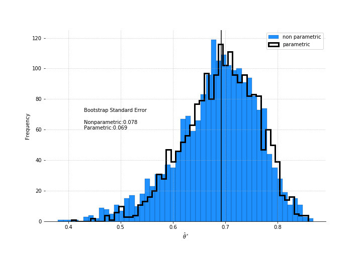
    all_fitted_vals[d] = np.array(fitted_vals).std(axis=0, ddof=1)

Let’s see what +/- 1.96$\hat{se}$ looks like².

What if we had done it non-paramterically?

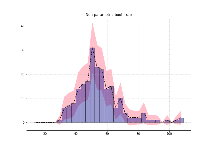
Increasing the degrees of freedom (df) of the fit increases the standard error. As df approaches 32, the number of bins, the standard errors approach the non-parametric one. So again, “nonparametric” just means “very high parameterised”.

Example: The “eigenratio”: take 2

We can apply the non-parametric method to the eigenratio problem as well. The distributional assumption here is that the sample comes from a 5-dimensional multivariate normal:

where $n$ is the number of students. We can draw a bootstrap sample:

where $\bar{x}$ and $\hat{\Sigma}$ are MLEs of the mean and covariance of the data.

The code is pretty straightforward:

def eigenratio2(arr):
    corr_mat = np.corrcoef(arr, rowvar=False)
    eig_vals, _ = eig(corr_mat)
    return np.max(eig_vals)/np.sum(eig_vals)

# MLE estimates
mean = data.mean().values
covar = np.cov(data, rowvar=False)

# draw bootstrap samples
samples = np.random.multivariate_normal(mean, covar, size=(2000, len(data)))

# get estimate for each sample
eigr_ls = []
for sample in tqdm(samples):
    eigr_ls.append(eigenratio2(sample))

As before, we get a smaller estimate for the SE than if used the non-parametric method.

Influence Functions, Robust Estimation, and the Bootstrap

Check out this data

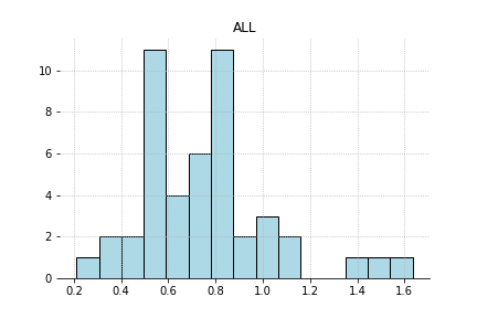
It has a little bit of a heavy tail. Would it be more efficient to estimate the center of the distribution by trimming the extreme values and then taking a mean? When you have a heavy tailed distribution, those tail have a large influence on your mean. Let’s formalise this a bit.

Say you have a sample $\boldsymbol{x} = (x_1, x_2, … , x_n)$ from some unknown distribution $F$. The influence function (IF) of some statistic evaluated at a point $x$ in $\mathcal{X}$, is the differential effect of modifying F by putting more probability on $x$.

$\delta_x$ is puts probability 1 on $x$ (and zero everywhere else). You’ll note that this is basically taking the gradient of your statistic over $\epsilon$. Let’s do this for the mean:

Plugging these into our formula for $\text{IF}(x)$:

The last line looks like hocus-pocus but it’s basically taking the derivative with respect to $\epsilon$. So the farther away $x$ gets from the mean, the more influence it has. This should agree with your intuition about means. So if $F$ is heavy tailed, your estimate would be very unstable.

These “unbounded” IFs make $\bar{x}$ unstable. One thing we can do is to calculate the trimmed mean. We throw away the portion of $F$ that is above a certain percentile. What does bootstrap tell us about the standard error if we do this?

Here’s are functions to trim and get the IF:

def get_IF(data_sr, alpha):
    """ Get Influence function when trimmed at alpha """
    low_α = np.percentile(data_sr, alpha*100,
                                  interpolation = 'lower')
    high_α = np.percentile(data_sr, (1-alpha) * 100,
                                  interpolation = 'higher')   
    mask_low = (data_sr < low_α)
    mask_high = (data_sr > high_α)

    vals = data_sr.copy()
    vals[mask_low] = low_α
    vals[mask_high] = high_α

    return (vals - vals.mean()) / (1 - 2*alpha)


def get_trimmed(data_sr, alpha):
    """ Get the trimmed data """
    low_α = np.percentile(data_sr, alpha*100,
                                  interpolation = 'higher')
    high_α = np.percentile(data_sr, (1-alpha) * 100,
                                  interpolation = 'lower')  

    mask02_low = (data_sr < low_α)
    mask02_high = (data_sr > high_α)

    return data_sr[~(mask02_low | mask02_high)]

where alpha is the percentage at the ends that we want to trim away. For different levels of alpha we can get a mean and a bootstrapped sd:

mean_tr = []
mean_if = []
res = []
for α in [0, 0.1, 0.2, 0.3, 0.4, 0.5]:
    mean_tr = []
    mean_if = []
    for i in range(1000):
        sample= np.random.choice(data_all, size=len(data_all))
        trimmed_sample = get_trimmed(sample, α)
        mean_tr.append(trimmed_sample.mean())
        N = len(trimmed_sample)
        mean_if.append(get_IF(sample, α).std()/np.sqrt(len(data_all)))
    res.append({"Trim":α,
                "Trimmed Mean": np.mean(mean_tr),
                "Bootstrap sd":np.std(mean_tr),
                "IFse":np.mean(mean_if)})

Let’s look at the results:

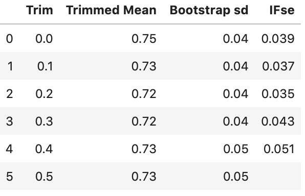
The bootstrap standard error for our sample mean is the smallest with an alpha of 0.2. We might be better off using a trim of 0.2 than no trim.

Conclusions

Do a bootstrap. Go parametric if you can. Use bootstrap to figure out the more efficient estimator.

Check out the notebook for all the code here.

Footnotes

¹ Yes - i know, only for homoscedastic errors.

² if you’re looking for confidence intervals, this is not a great way to do it. It assumes normality for each of the estimates which is obviously not true – support is only positive numbers. Bias corrected confidence intervals are explored in Chapter 11 of CASI.