In this post, I just implement a Gibbs and a slice sampler for a non-totally-trivial distribution. Both of these are vanilla version – no overrelaxation for Gibbs and no elliptical slice samplers, rectangular hyper-boxes etc. I am hoping you never use these IRL. It is a good intro though.
Generating the data
Instead of the usual “let’s draw from a 1-d gaussian” example, let’s make our samplers work a bit. We’re going to generate a mixture of three 2-d gaussians where the dimensions are correlated.
The following class creates such a distribution
class GaussianMix(object):
def __init__(self, n_clusters, n_dims, means=None, cov=None, low=-3, high=3):
if means == None:
means = np.random.randint(low=low, high=high, size=(n_clusters, n_dims))
elif (means.shape[0] != n_clusters) or (means.shape[0] != n_dims):
raise RuntimeError("Incorrect dimensions for means")
if cov == None:
cov = np.empty((n_clusters, n_dims, n_dims))
for i in range(cov.shape[0]):
corr = st.random_correlation.rvs(np.random.dirichlet(alpha = np.ones(n_dims)) * n_dims)
sig = np.random.uniform(low=1, high=(high-low)/2, size=n_dims)
cov[i] = corr * sig.reshape(-1, 1) * sig
elif (cov.shape[0] != n_clusters) or (cov.shape[1] != n_dims) or (cov.shape[2] != n_dims):
raise RuntimeError("Incorrect dimensions for cov")
self.means = means
self.cov = cov
self.n_clusters = n_clusters
self.n_dims = n_dims
def rvs(self, size=100):
all_points = []
for dim in range(self.n_clusters):
points = st.multivariate_normal(self.means[dim], self.cov[dim]).rvs(size)
all_points.append(points)
return np.row_stack(all_points)
def pdf(self, x):
pdf_val = 0
for dim in range(self.n_clusters):
pdf_val += st.multivariate_normal(self.means[dim], self.cov[dim]).pdf(x)
return pdf_val / self.n_clusters
def get_weights(self, point, dim):
distance = np.zeros(self.n_clusters)
other_dims = np.delete(np.arange(self.n_dims), dim).squeeze()
point_other_dim = point[other_dims]
for i in range(self.n_clusters):
distance[i] = st.norm(self.means[i][other_dims], self.cov[i][other_dims][other_dims]).pdf(point_other_dim)
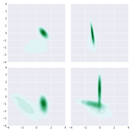
return distance / distance.sum()Let’s use this to generate a few different distribution to see what they look like.
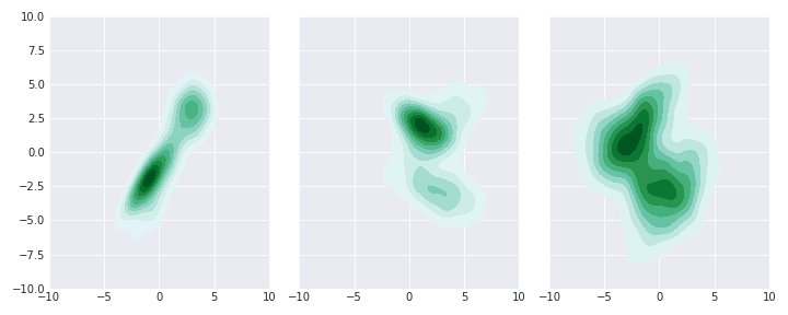
So, not easy ones; Some islands, some covariance, some corner. Now let’s write our samplers.
Slice sampler
Here’s a 2d slice sampler - we create two auxiliary variables. The code is based off the pseudo-code in Mackay’s book. Note that the proposal boxes are squares and shrunk at the same rate. Not great since we know there is a lot of covariance. In a later post, we might check out some of the more advanced techniques to improve our proposal.
def get_interval(x, dist, u, w = 0.1):

    r = np.random.uniform(0, 1)
    xl = x - r*w
    xr = x + (1 - r) * w

    while (dist.pdf(xl) > u).any():
        xl = xl - w

    while (dist.pdf(xr) > u).any():
        xr = xr + w

    return xl, xr

def modify_interval(x, x_prime, xl, xr):

    dims = x.shape[0]
    for d in range(dims):
        if x_prime[d] > x[d]:
            xr[d] = x_prime[d]
        else:
            xl[d] = x_prime[d]

    return xl, xr

def slice_sampler2d(dist, n=1000, x_init = np.array([2, 1]), w = 0.5):

    x_prime = x_init
    all_samples = []
    n_samples = 0

    dim = np.shape(x_init)[0]

    while n_samples < n:

        # evaluate P*(x)
        p_star_x = dist.pdf(x_prime)

        # draw a vertical u' ~ U(0, P*(x))
        u_prime = np.random.uniform(0, p_star_x, size=2)

        # create a horizontal interval (xl, xr) enclosing x
        xls, xrs = get_interval(x_prime, dist, u_prime, w=w)

        # loop
        break_out = True

        iters = 0
        x_old = x_prime
        while break_out and (iters <= 1000):
            # draw x' ~ U(xl, xr)
            x_prime = np.random.uniform(xls, xrs)

            # evaluate P*(x')
            p_star_x = dist.pdf(x_prime)

            # if P*(x') > u' break out of loop
            if (p_star_x > u_prime).all():
                break_out = False

            # else modify the interval (xl, xr)
            else:
                xl, xr = modify_interval(x_old, x_prime, xls, xrs)
            iters += 1
            if iters == 1000:
                print("!!! MAX ITERS")
        all_samples.append(x_prime)
        n_samples += 1

    return np.row_stack(all_samples)
Let’s see how it does for the last example distribution above.
samples_slice = slice_sampler2d(dist, x_init=np.array([-4, 0]), n=10000, w=10)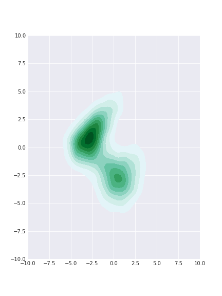
Not bad! Generally the right shape though the lower island seemed to have been sampled less. We also seemed to have sufficient samples from the middle of the distribution but the tail samples seems to be missing.
Gibbs sampler
We need to the conditionals for the Gibbs sampler. Since we are working with multivariate normals, that easy.
def gaussian_conditional(mu, cov, dim, dim_vals):

    # roll axis to get the dimension of interest to the top
    sig = np.roll(np.roll(cov, -dim, axis=0), -dim, axis=1)

    mu_2 = np.delete(mu, dim)
    mu_1 = mu[dim]

    sig_11 = sig[0, 0]
    sig_12 = sig[0, 1:]
    sig_21 = sig[1:, 0]
    sig_22 = sig[1:, 1:]

    sig_22_inv = np.linalg.pinv(sig_22)

    mu_bar = mu_1 + sig_12 @ sig_22_inv @ (dim_vals - mu_2)
    sig_bar = sig_11 - sig_12 @ sig_22_inv @ sig_21

    return mu_bar, np.sqrt(sig_bar)
The tricky part is picking which gaussian conditional to draw from. Remember that we have 3 multivariate gaussians. So any given point could have come from any of those three. But we know how likely it is that they came from each of those. We can just use these as weights and draw from a multinomial to pick conditional distribution.
The code to get the weights is already included in the GaussianMix class above. Here’s the code for the sampler.
def gibbs_sampler_mix(gm, init=[0.0, 1.0], n_samples = 1000):

    dim_vals = np.array(init, dtype='float')
    samples = []
    n_dims = gm.n_dims

    for i in range(n_samples):
        for dim in range(n_dims):
            if dim == (n_dims - 1):
                next_dim = 0
            else:
                next_dim = dim + 1

            cond_vals = np.delete(dim_vals, dim)

            weights = gm.get_weights(dim_vals, dim)
            c_id = st.multinomial(1, weights).rvs()
            cluster_id = np.argmax(c_id)

            mu_bar, sig_bar = gaussian_conditional(gm.means[cluster_id],gm.cov[cluster_id], dim, cond_vals)

            dim1_sample = np.random.normal(mu_bar, sig_bar)
            dim_vals[dim] = dim1_sample
            samples.append(dim_vals.copy())

    return np.row_stack(samples)
Let’s draw!
samples_gibbs = gibbs_sampler_mix(dist, init=[0, 0], n_samples = 10000)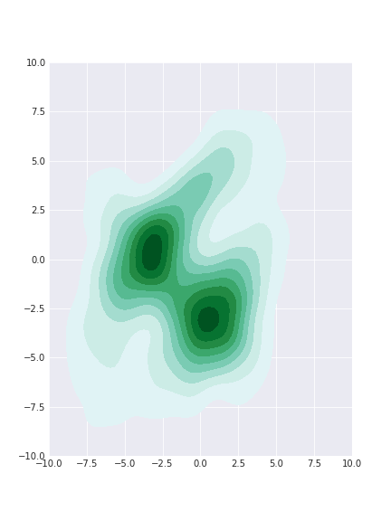
We burned the first 5000 samples and plotted the rest. Now we have plenty of samples (too many?) from the tails and the shape of the core is still approximately correct.
Comparison
We can do better than visual inspection though. Let’s just generate a 1000 different distributions and compare the KL divergence across a marginal between the samples from GaussianMix and samples from the two samplers.
I’ve trimmed the values greater than 1.0 for readability.
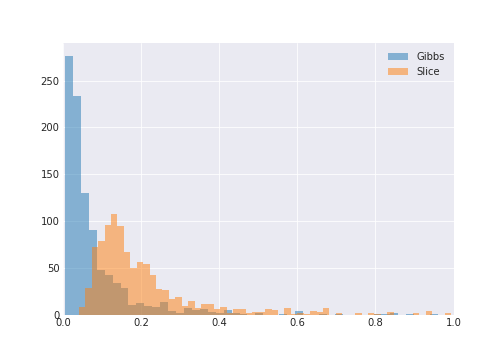
So Gibbs does better than slice with lower KL divergence scores. But not always.
Here are some where Gibbs does better than slice:
And some where slice does better than Gibbs:
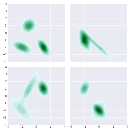
For multimodal distributions, slice does better than Gibbs. There may be a better Gibbs sampler that overcomes this but this makes sense for our implementation. The multinomial draw is very unlikely to shift you to the other far away gaussians if you stuck in one.
So if you have little covariance and the distribution is unimodal (and you have the conditionals!) the Gibbs rocks it. The covariance thing is not a deal breaker though (see overrelaxation) but not sure how I’d get over the multimodal problem in my example.