Following David Mackay’s book along with his videos online has been a real joy. In lecture 11, as an example of an inference problem, he goes over many variations of the k-means algorithm. Let’s check these out.
The datasets
All the sample data used in his lectures and the book can be found on his website here. It also has octave code for the algorithms but we’ll implement them again in python.
The simple k-means
This is now a classic data science interview question and you probably know how to do this in your sleep. Here’s my simple implementation of it. You can make this a lot more efficient by using numpy’s vectorized functions but I don’t bother with it here.
def assigment_step(centroids, xs):

    assignments = []

    for x in xs:
        best_centroid = 0
        best_distance = np.inf
        for c_id, c in enumerate(centroids):
            x_to_c = sp.spatial.distance.euclidean(x, c)
            if x_to_c < best_distance:
                best_centroid = c_id
                best_distance = x_to_c

        assignments.append(best_centroid)

    return np.array(assignments)


def update_step(xs, assignments, n):

    all_centroid = []

    for i in range(n):
        i_idx = np.argwhere(assignments == i).squeeze()
        assigned_xs = xs[i_idx].reshape(-1, 2)
        centroid = np.sum(assigned_xs, axis = 0) / assigned_xs.reshape(-1, 2).shape[0]
        all_centroid.append(centroid)
    return np.row_stack(all_centroid)
and here’s the code that runs the simulation which doesn’t change much between the different versions so we’ll skip it going forward.
def run_simulation(xs, n_clusters):

    # We don't want to intialize two clusters to the same point
    unique_xs = np.unique(xs, axis=0)

    # initialize clusters
    centroids_idx = np.random.choice(np.arange(unique_xs.shape[0]), size=n_clusters, replace=False)
    new_centroids = unique_xs[centroids_idx]
    prev_centroids = np.zeros_like(new_centroids)

    assignments = assigment_step(new_centroids, xs)
    iteration = 0

    while not np.isclose(new_centroids, prev_centroids, atol=1e-10, rtol=1e-8).all():

        prev_centroids = new_centroids
        new_centroids = update_step(xs, assignments, n_clusters)
        assignments = assigment_step(new_centroids, xs)

        iteration += 1

    assignments2 = np.invert(assignments, dtype=np.int8) + 2
    assignments = np.column_stack([assignments2, assignments])

    return assignments, new_centroids, []
We’re going to look at the 7 different datasets and see how this code does in picking up the clusters.
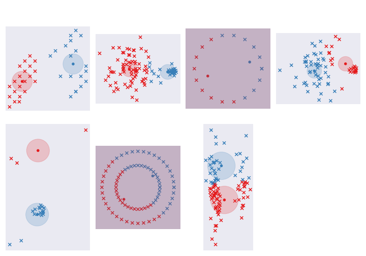
It does a fine job with the first ones but struggles with the rest. One problem is that we dichotomize the allocation for each point - it either belongs to cluster 1 or cluster 2. Some points may be ambiguous and we want to take that into account. Let’s fix that in the next section.
Simple k-means with soft-thresholding
Now each cluster has a “responsibility” for each point. The total responsibility for a point adds up to 1. We do a softmax instead of the hard threshold in the assignment step. And when updating the cluster center, we weight the points based on this responsibility.
def assignment_step_soft(centroids, xs, beta):

    assignments = []

    distance_to_centroids = np.zeros((xs.shape[0], centroids.shape[0]))

    for x_id, x in enumerate(xs):
        for c_id, c in enumerate(centroids):
            distance_to_centroids[x_id, c_id] = -beta * sp.spatial.distance.euclidean(x, c)

    return softmax(distance_to_centroids, axis=1)

def update_step_soft(xs, assignments, n):

    all_centroid = []

    for i in range(n):
        centroid_resps = assignments[:, i]
        centroid = centroid_resps @ xs / centroid_resps.sum()
        all_centroid.append(centroid)

    return np.row_stack(all_centroid)
Note the new parameter beta that we now need to set. The higher the beta, the more hard the thresholding. In its limit, it approaches the basic k-means algorithm.
Here are the results with beta set to 2:
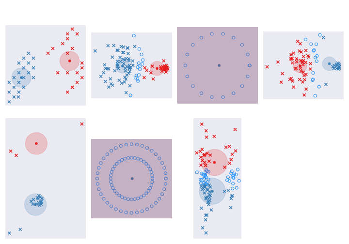
Do we do any better? Well, not really. Though we are able to identify the ones we are uncertain about - the circles in light-blue - we now have an additional parameter, beta, to set. The other limitation of the algorithm is that each cluster is assumed to be the same size. We see from the data that this is not always true. Let’s allow for variable sizes in the next section.
K-means with variable cluster sizes
Now we are going to think of each cluster as a gaussian. They can be of varying sizes i.e. different variances. So the distance of each point to the gaussian center is the likelihood of observing that point given the gaussian parameters weighted by the cluster’s importance (pi). And what is importance? The total amount of relative responsibility of the cluster across all the points.
def gaussian_dist(c, sigma, x, pi):

    responsibility = pi * sp.stats.multivariate_normal(mean=c, cov=np.array([[sigma**2, 0],[0, sigma**2]])).pdf(x)
    return responsibility
So we are still keeping the idea of responsibility around but look ma, no beta!. Our update and assignment steps now need to keep track of importance and also update the variance or size for each of the clusters.
def assignment_step_softv2(centroids, xs, sigmas, pis):

    assignments = []

    distance_to_centroids = np.zeros((xs.shape[0], centroids.shape[0]))

    for x_id, x in enumerate(xs):
        for c_id, c in enumerate(centroids):
            sigma = sigmas[c_id]
            pi = pis[c_id]
            distance_to_centroids[x_id, c_id] = gaussian_dist(c, sigma, x, pi)

    normed_distances = distance_to_centroids / distance_to_centroids.sum(axis=1).reshape(-1, 1)
    normed_distances[np.isnan(normed_distances)] = 0

    return normed_distances

def update_step_softv2(xs, assignments, n, curr_sigmas, curr_centroids):

    all_centroid = []
    all_sigma = []

    for i in range(n):
        centroid_resps = assignments[:, i]

        curr_sigma = curr_sigmas[i]
        curr_centroid = curr_centroids[i,:]

        total_resp = centroid_resps.sum()

        if total_resp == 0:
            all_centroid.append(curr_centroid)
            all_sigma.append(curr_sigma)
            print("no resp for cluster %s" % str(i))
        else:
            # m
            centroid = centroid_resps @ xs / total_resp

            # sigma
            sigma = (centroid_resps @ ((xs - centroid) ** 2).sum(axis=1)) / (xs.shape[1] * total_resp)

            if sigma == 0:
                sigma = 0.1

            all_centroid.append(centroid)
            all_sigma.append(np.sqrt(sigma))

    # pi
    pi = assignments.sum(axis=0) / assignments.sum()

    return np.row_stack(all_centroid), np.array(all_sigma), pi
The update step suddenly looks quite long. This is because, we need to handle the corner cases where a cluster has no importance or has just one point assigned to it, reducing the variance to almost zero. The algorithm falls over during those scenarios. We don’t change the cluster details if it has no importance and if sigma shrinks to zero, we set it to something small - 0.1 in this case. You may have more elegant ways of handling this.
So what did we get for all this hard work?
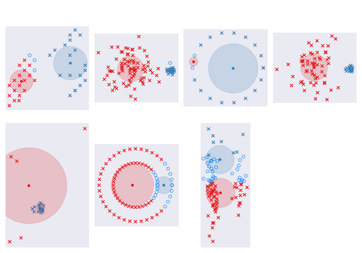
Good news is that all the ambiguity in the second and fourth dataset is now gone - we have a small cluster and a large cluster. Bad news is that there is a little more ambiguity about the some of the peripheral points in the first dataset since the blue cluster is now larger and more important. It still does a shitty job of the circles and the last dataset with skinny clusters.
We can’t do much about the circles unless we change coordinate systems / do some transformations and I’ll leave that out for now (another reason to use HDBSCAN or Spectral Clustering if this is a real life problem). But we can do something about the skinny clusters. So far we have kept the cluster round - i.e. the variance in the two dimensions are constrained to be equal. Let’s relax that in the next section.
K-means with adaptive covariance
I’m adding a try/except since the covariance matrix becomes invalid under some scenarios (the same ones as above). In these cases, we just pick a tiny round cluster.
def gaussian_dist_v4(c, cov, x, pi):

    try:
        responsibility = pi * sp.stats.multivariate_normal(mean=c, cov=cov).pdf(x)
    except np.linalg.LinAlgError as err:
        responsibility = pi * sp.stats.multivariate_normal(mean=c, cov=np.array([[0.01, 0],[0, 0.01]])).pdf(x)

    return responsibility
The assignment step is exactly the same as before. So let’s look at the update step.
def update_step_softv4(xs, assignments, n, curr_sigmas, curr_centroids):

    all_centroid = []
    all_sigma = []

    for i in range(n):
        centroid_resps = assignments[:, i]

        curr_sigma = curr_sigmas[i]
        curr_centroid = curr_centroids[i,:]

        total_resp = centroid_resps.sum()

        if total_resp == 0:
            all_centroid.append(curr_centroid)
            all_sigma.append(curr_sigma)
            print("no resp for cluster %s" % str(i))
        else:
            # m
            centroid = centroid_resps @ xs / total_resp

            # diag terms
            w_dist = xs - centroid

            # cov matrix
            cov_matrix = np.cov(w_dist.T, aweights=centroid_resps)
            cov_matrix = np.nan_to_num(cov_matrix)

            all_centroid.append(centroid)
            all_sigma.append(cov_matrix)

    # pi
    pi = assignments.sum(axis=0) / assignments.sum()

    return np.row_stack(all_centroid), np.stack(all_sigma), pi
Here are the results:
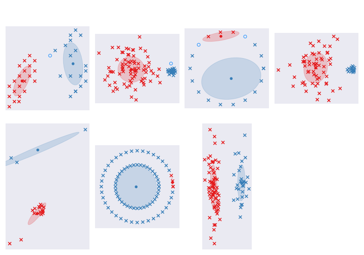
Not too bad, I think. Datasets 2 and 4 look ok. Circle ones are still rubbish. The last one with long clusters is perfect. Dataset 5 is a bit weird, but sure! That is valid way of clustering.
Conclusions
I cheated a little. EM algorithms tend to be sensitive to initial conditions. There is a lot of literature on how to handle that. If you are going to use this in real life for some insane reason, at least run it multiple times from different initial conditions to make sure it is stable. If not, take some sort of ensemble of all of them.
Here are all the results together.
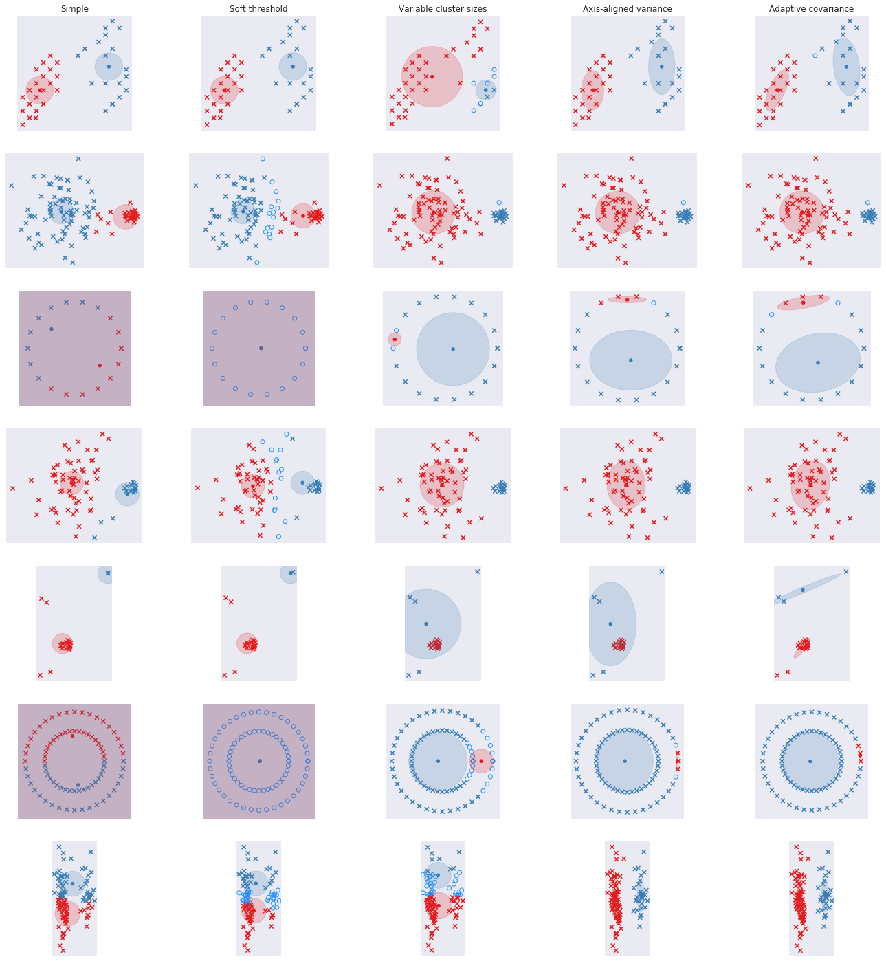
As always you can find the notebook with the code online. You may want to try these again with three clusters.