There are two ways of learning and building intuition. From the top down, like fast.ai believes, and the bottom up, like Andrew Ng’s deep learning course on coursera. I’m not sure what my preferred strategy is.
While learning Bayesian analysis, I’ve gone back and forth. David MacKay has a great lecture where he introduces Bayesian inference using a very small dataset of 8 data points. It was a cool way to introduce the topic so I decided to implement it. I learnt a tonne of stuff – not the least, animating 3d plots – doing it and refined my intuition. You can find the notebook here.
Problem setup
You have 8 data points as follows:
\[X = [ 0.64,\,0.016,\,0.1,\,0.05,\,3.09,\,2.14,\,0.2,\,7.1]\]We assume that this comes from one (or two) exponential processes.
We need to answer the following questions:
- What is the rate parameter assuming this comes from just one exponential process?
- What are the rate parameters assuming this comes from just two exponential processes?
- Which model, one process or two processes, is better supported by the data?
One process
First the easy stuff. Since it is an exponential, we can define likelihood, $P(x\vert\lambda)$, as
\[P(x|\lambda) = \prod_{i=1}^{8} \frac{1}{\lambda} exp(-\frac{\lambda}{x_i})\]$x$ is given, so let’s see what this looks like
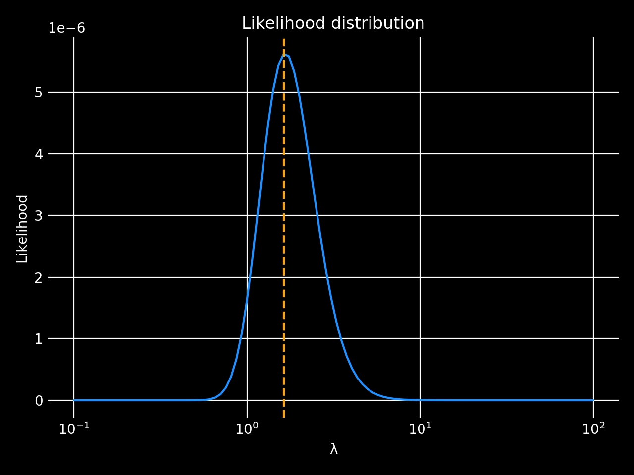
N.B: Why is the plot black? Idk. I spent too long replicating David Mackay’s style – then discovered that it is just the classic gnuplot colors. But it looks nice I think.
The blue line shows what lambda could be. If you pushed me for a point estimate, I might give you the MAP value which is shown by the orange line.
Note that we are assuming that all lambdas are equally likely (flat prior). We know that’s rubbish but let’s pretend for the sake of this exercise.
The evidence
The evidence is given by :
\[\begin{align} P(x) = \int_0^{\infty} P(x|\lambda)\, d \lambda \\ \hat{P}(x) = \sum_{i=1}^{N} P(x|\lambda_i)\,P(\lambda) \\ \hat{P}(x) = \frac{1}{N} \sum_{i=1}^{N} P(x|\lambda_i) \\ \end{align}\]That just taking the mean of all the likelihoods since we are assuming a flat prior on lambda:
evidence1 = all_likelihoods.mean()
Two processes
Now for the fun bit. What if we had two exponential processes, with rate parameters $\lambda_0$ and $\lambda_1$ respectively?
Let $k$ define the vector of assignment of each of the data points to one of the two processes. So $k_i$ == 1’s say we knew the process assignments $k$. So for example, $k$ could be $[1\, 0\, 0\,0\,0\,1\,1\,1]$ which says that the first and the last three points come from process 2 while the rest come from process 1. If we do know $k$, we can calculate the likelihood as follows:
\[\begin{aligned} P(\mathbf{x}|\lambda_0, \lambda_1, \mathbf{k}) &= \prod_{i=1}^{8} \frac{1}{\lambda_{k_i}} exp(-\frac{\lambda_{k_i}}{x_i}) \end{aligned}\]So for a given vector $k$, we can get the likelihood for all combinations of $\lambda_0$ and $\lambda_1$. Since $\vert k \vert$ is 8, there are $2^8$ possible $k$ vectors. We can just iterate over all of these $k$ vectors and calculate the likelihood. The seizure-inducing gif below shows the likelihood for all combinations of $\lambda_0$ and $\lambda_1$ for every possible $k$ - all $2^8$ of them.
Mackay asks us to imagine these as a stack of pancakes. So each pancake is $P(\mathbf{x}\vert \lambda_0, \lambda_1, \mathbf{k})$ for a possible value of $\mathbf{k})$.
Now what we really want is $P(x \vert \lambda_1, \lambda_2)$ which is:
\[\begin{aligned} P(\mathbf{x}|\lambda_0, \lambda_1) &= \int P(\mathbf{x}|\lambda_0, \lambda_1, \mathbf{k})\,d\mathbf{k}\\ \hat{P}(\mathbf{x}|\lambda_0, \lambda_1) &= \frac{1}{2^8}\sum_k P(\mathbf{x}|\lambda_0, \lambda_1, \mathbf{k}) \end{aligned}\]So all you need to do is take an average of all the pancakes.
This is also the posterior distribution if you:
- Assume every $k$ has equal probability i.e. probability of each point belonging to a process is $\frac{1}{2}$ and each $k$ vector has probability $\frac{1}{2^8}$. Not that outrageous an assumption.
- Normalize
And you get this:
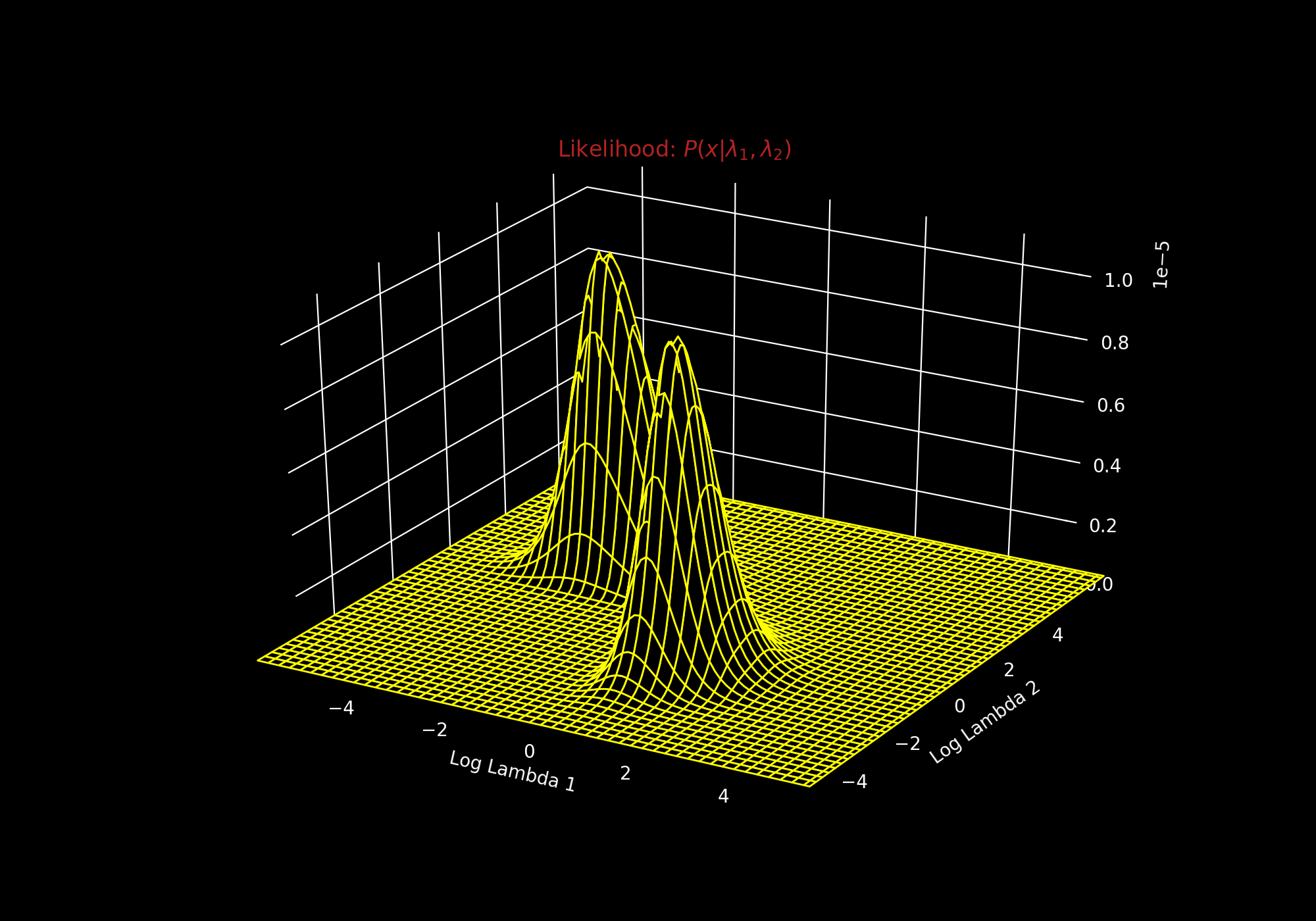
We get two distinct peaks, so there are indeed two distinct exponential processes. And if you wanted to know the best process assignment vector, $\mathbf{k}^* $, you could just look at the maximum likelihood for each $\mathbf{k}$ and normalize.
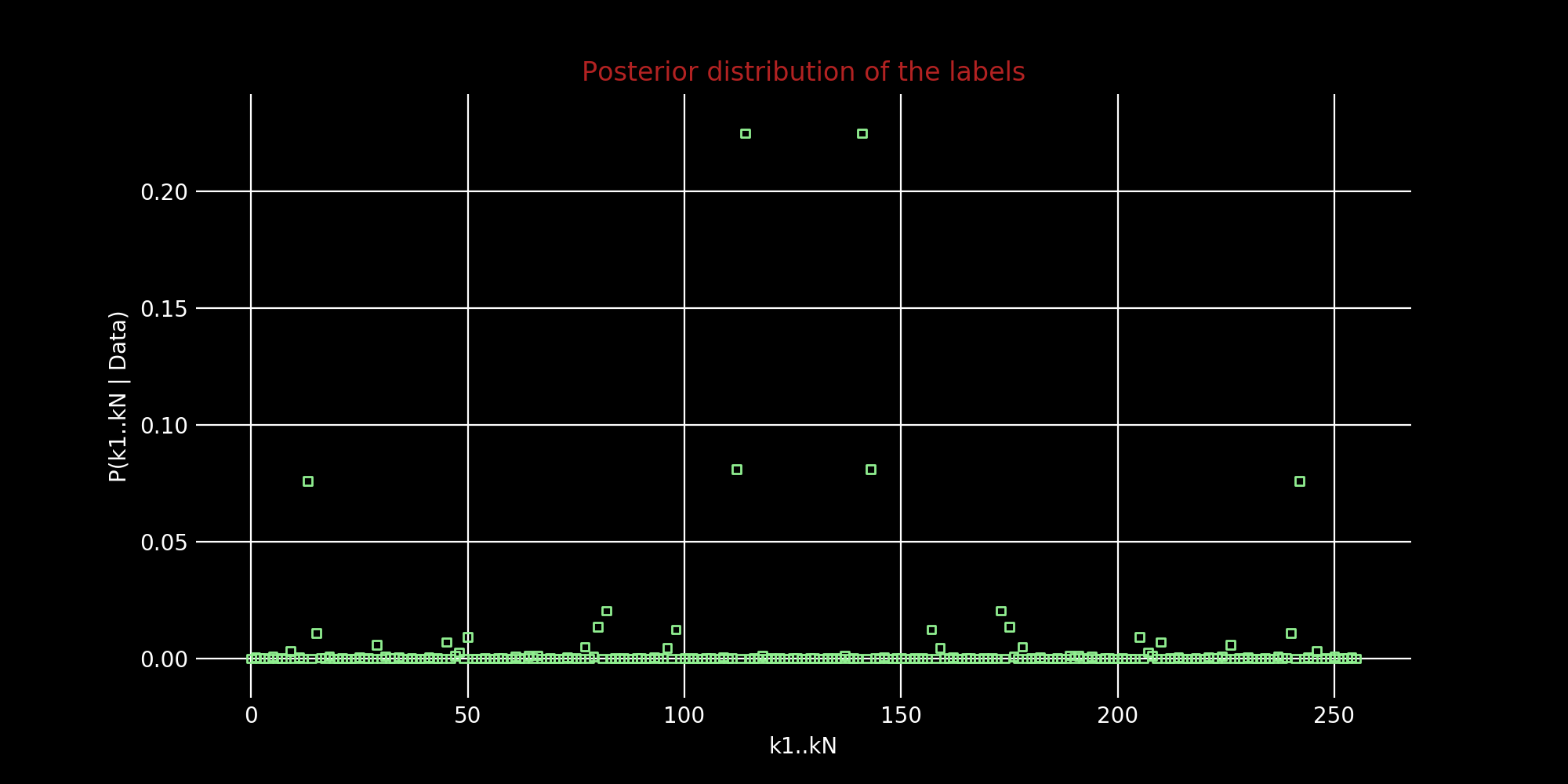
Wunderbar! So the best k is 114 or $[0, 1, 1, 1, 0, 0, 1, 0]$ and its twin 141 or $[1, 0, 0, 0, 1, 1, 0, 1]$ depending if $\lambda_0$ > $\lambda_1$ or $\lambda_1$ > $\lambda_0$. Label-switching is pretty annoying when working with mixture models. We won’t worry about it here and just pick one.
The evidence
The same formula for evidence applies here. We have some the extra $\mathbf{k}$ paramters but that’s no worry for us since we are assuming flat priors on it as well. So we’ll just take the mean over all the parameters and Bob’s your uncle
evidence2 = all_Z.mean()
evidence2
Comparing Models
In previous posts we have used WAIC to compare models. We’ll do something simpler (and terrible depending on who you ask) - we’ll just calculate the Bayes Factor. The ratio of the evidences is just
evidence2 / evidence1
which is around 13 for our data. Since it’s substantially greater than 1, we conclude that model 2, with two processes, fits the data better.
There’s another way to look at this. Let $H_1$ be the hypothesis that there is just one process and $H_2$ be the hypothesis that there are two processes. A priori we think both of these hypothesis are equally likely:
\[p(H_1) = p(H_2) = 0.5\]So posterior for $p(H_1 \vert x)$ is just:
\[p(H_1 \vert x) = \frac{p (x | H_1) \cdot p (H_1)}{p (x | H_1) \cdot p (H_1) + p (x | H_2) \cdot p (H_2)}\]This just boils down to:
PosteriorProbOfH2 = evidence2  / (evidence1 + evidence2)
PosteriorProbOfH1 = evidence1  / (evidence1 + evidence2)
which gives:
\[\begin{align} p(H_2 \vert x) = 0.93 \\ p(H_1 \vert x) = 0.07 \end{align}\]Conclusion
So looks like $H_2$, that there are two processes is better supported by the data. Feel free to check out the notebook for all the code and to see what the MAP values for the $\lambda$ work out to be.