If you want to measure the causal effect of a treatment what you need is a counterfactual. What would have happened to the units if they had not got the treatment? Unless your unit is Gwyneth Paltrow in Sliding Doors, you only observe one state of the world. So the key to causal inference is to reconstruct the untreated state of the world. Athey et al. in their paper show how matrix completion can be used to estimate this unobserved counterfactual world. You can treat the unobserved (untreated) states of the treated units as missing and use a penalized SVD to reconstruct these from the rest of the dataset. If you are familiar with the econometric literature on synthetic controls, fixed effects, or unconfoundedness you should definitely read the paper; it shows these as special cases of matrix completion with the missing data of a specific form. Actually, you should read the paper anyway. Most of it is quite approachable and it’s very insightful.

Also, check out this great twitter thread by Scott Cunningham and Cyrus Samii’s notes] on it.

Data setup

Say you have some panel data with $N$ units and $T$ time periods. At some time period $t_{0,n}$ (which can be different for each unit), some of the units get the treatment. So from $(t_{0,n}, T)$ you don’t really see the untreated state of the world. It is “missing”. We’ll use the same dataset, the Abadie 2010 California smoking data, that the authors use in the paper for the demo:

import numpy as np
import pandas as pd
import scipy as sp

import seaborn as sns
import matplotlib.pyplot as plt

from tqdm import tqdm_notebook as tqdm

BASE_URL = "https://raw.githubusercontent.com/susanathey/MCPanel/master/tests/examples_from_paper/california/"
Y = pd.read_csv(BASE_URL + "smok_outcome.csv", header=None).values.T
Y = Y[1:,:]  # drop the first row since it is treated and the untreated values for that unit are not available.

N, T = Y.shape

Let’s allow each unit to have a different $t_0$ with the minimum being 16 and pick 15 random units to be treated.

t0 = 16

N_treat_idx = np.random.choice(np.arange(N), size = 15, replace=False)
T_treat_idx = np.random.choice(np.arange(t0, T), size = 15, replace=False)

treat_mat = np.ones_like(Y)

for n, t in zip(N_treat_idx, T_treat_idx):
    treat_mat[n, t:] = 0

What we will observe is Y_obs:

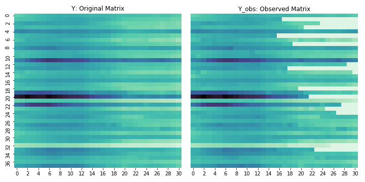
Y_obs = Y * treat_mat

and we’ll try and recreate Y. The figure below shows what these datasets look like. The white bits on the right are the “missing” entries in the matrix.

The algorithm

Our job is to reconstruct a matrix $L$ such that:

Before we get to the estimator for $L^* $, let’s define a few support functions:

where $\mathbf{\tilde{\Sigma}}$ is equal to $\mathbf{\Sigma}$ with the i-th singular value $\sigma_i(\mathbf{A})$ replaced $\text{max}(\sigma_i(\mathbf{A}) - \lambda, 0)$. So you are doing a SVD and shrinking the eigenvalues towards zero. Here’s the python code for it:

def shrink_lambda(A, lambd):

    S,Σ,R = np.linalg.svd(A, full_matrices=False)
    #print(Σ)

    Σ = Σ - lambd
    Σ[Σ < 0] = 0

    return S @ np.diag(Σ) @ R

And then

In python:

def getPO(A, O):

    A_out = np.zeros_like(A)
    A_out[tuple(O.T)] = A[tuple(O.T)]

    return A_out

def getPOinv(A, O):

    A_out = A.copy()
    A_out[tuple(O.T)] = 0

    return A_out

And now for the main algorithm. The paper shows the general form of the estimator but here we will implement the iterative (probably slower) version. It’s quite beautiful in its simplicity. For $k = 1,2,…,$ define:

and we initialize it as

Note that $\mathscr{O}$ is the set of coordinates of the matrix where the data is not missing i.e. the units were not treated.

We run this until $\mathbf{L}$ converges. Here’s the python code:

def run_MCNNM(Y_obs, O, lambd = 10, threshold = 0.01, print_every= 200, max_iters = 20000):

    L_prev = getPOinv(Y_obs, O)
    change = 1000
    iters = 0

    while (change > threshold) and (iters < max_iters):
        
        PO = getPO(Y_obs, O)
        PO_inv = getPOinv(L_prev, O)

        L_star = PO + PO_inv
        L_new = shrink_lambda(L_star, lambd)

        change = np.linalg.norm((L_prev - L_new))

        loss = ((Y_obs - L_new) ** 2).sum() / Y.sum()
        real_loss = ((Y - L_new) ** 2).sum() / Y.sum()

        L_prev = L_new
        iters += 1

        if (print_every is not None) and ((k % print_every) == 0):
            print(loss, change, real_loss)

    return L_new

Cross-validation

We still need to figure what $\lambda$ needs to be so we cross-validate. The implementation below is not perfect since it doesn’t simulate the full dataset exactly. I’m picking a random subset of coordinates to take out as the test set and training using the rest. I’m not removing everything after a some time $t$ for each unit as I really should. Check out the note in the paper on cross validation for $\lambda$. But the implementation below should give you a good sense (and a good start if you want to improve it) of how to do it. While you’re at it, you may want to use dask distributed to parallelize it.

from sklearn.model_selection import KFold

def get_CV_score(Y_obs, O, lambd, n_folds = 4, verbose=False):

    kfold = KFold(n_splits=n_folds, shuffle=True)

    mse = 0
    for i, (Otr_idx, Otst_idx) in enumerate(kfold.split(O)):
        Otr = O[Otr_idx]
        Otst = O[Otst_idx]
        if verbose: print(".", end="")

        L = run_MCNNM(Y_obs, Otr, lambd, threshold = 1e-10, print_every= 15000, max_iters = 20000)

        mse += ((Y_obs[tuple(Otst.T)] - L[tuple(Otst.T)]) ** 2).sum()

    return mse / n_folds

def do_CV(Y_obs, O, lambdas = [5, 10, 20, 40], n_tries = 10, verbose=False):

    score = {}

    for t in tqdm(range(n_tries)):
        run_score = {}
        for l in tqdm(lambdas, leave=False):
            if verbose: print(f"lambda {l}:", end="")
            run_score[l] = get_CV_score(Y_obs, O, l, n_folds = 4, verbose=verbose)
            if verbose: print(f" : {run_score[l]}")
        score[t] = run_score
    return score

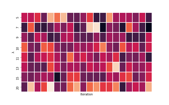
Let’s run the cross-validation and check out the results:

cv_score = do_CV(Y_obs, O, lambdas=[5, 7, 9, 10, 11, 13, 15, 20], n_tries = 20)
cv_score_df = pd.DataFrame(cv_score)

plt.figure(figsize=(8, 5))
ax = sns.heatmap(cv_score_df, linewidths=1, cbar=False)
ax.set_xticks([]);

ax.set_xlabel("Iteration")
ax.set_ylabel("λ")
plt.savefig("../../sidravi1.github.io/assets/2018_12_02_cross_val.png")

cv_score_df.mean(axis=1)

Here are the results (darker is smaller MSE) and it looks like 9 is the optimal lambda.

Final run and results

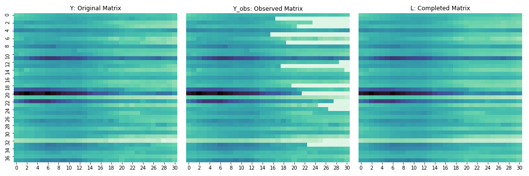
Using 9 as our lambda, let’s run it once more and check out the results.

lambd = 9
threshold = 1e-10
O = np.argwhere(treat_mat)

L = run_MCNNM(Y_obs, O, lambd, threshold, print_every= 1000, max_iters = 20000)

# plot the results

vmin = Y.min()
vmax = Y.max()

f, (ax1, ax2, ax3) = plt.subplots(1, 3, figsize=(15, 5))
sns.heatmap(Y, linewidths=0, vmax=vmax, vmin=vmin, ax = ax1, cmap = 'mako_r', cbar=False)
ax1.set_title("Y: Original Matrix")

sns.heatmap(Y_obs, linewidths=0, vmax=vmax, vmin=vmin, ax = ax2, cmap = 'mako_r', cbar=False)
ax2.set_title("Y_obs: Observed Matrix")
ax2.set_yticks([])

sns.heatmap(L, linewidths=0, vmax=vmax, vmin=vmin, ax = ax3, cmap = 'mako_r', cbar=False)
ax3.set_title("L: Completed Matrix")
ax3.set_yticks([])


plt.tight_layout()

plt.savefig("../../sidravi1.github.io/assets/2018_12_02_athey_reconstructed.png")

Not bad at all! Looks like we lost some resolution there but we only had 38 records so pretty decent. I bet with a larger dataset with more controls, it would do even better.

Next steps

We don’t include any covariate here but the paper shows how you can do that. Athey and team has also made their code and test data available online which deserves a round of applause. It is still such a rare thing in economics. You can go check out their code here. It also includes a R package which will be a hell of a lot faster than my quick and dirty code.

The notebook with all my code can be found here. Happy matrix completing!