David McKay’s Information Theory, Inference, and Learning Algorithms, in addition to being very well written and insightful, has exercises that read like a book of puzzles. Here’s one I came across in chapter 2:

Excercise 2.35 Fred rolls an unbiased six-sides die once per second, noting the occasions when the outcome is a six.
(a) What is the mean number of rolls from one six to the next six?
(b) Between two rolls, the clock strikes one. What is the mean number of rolls until the next six?
(c) Now think back before the clock struck. What is the mean number of rolls, going back in time, until the most recent six?
(d) What is the mean number of rolls from the six before the clock struck to the next six?
(e) Is your answer to (d) different from the your answer to (a)? Explain.

(a) is easy enough. Anyone who has played any game requiring dice will tell you it’s 6.
(b) may seem a little puzzling to some. When people ask “what’s the clock striking one got to do with it?”, I put on a devilish grin and saying “Nothing!”. But if you are familiar with Poisson processes, you have heard this sort of stuff many times. You note that throws are memoryless i.e. Probability of a 6 in throw $T$. $P(T)$ does not depend on any throws $t$ where $t < T$. And you say, “These throws are memoryless so it is still 6”. And you’d be right (even my mum, who is not a student of probability, got it right).
For (c) you are thinking “Ok so it’s memoryless. Does directionality of time matter? It really shouldn’t right?” and you again correctly guess 6.
(d) leads you down a trap; you add the two together and minus one (so you aren’t counting the 1/2 second) and say 11.
(e) Closes the trap on you. Just because an unrelated event like a clock striking one happened, why should the expected number of rolls be almost double?

McKay doesn’t directly provide a solution but instead cheekily just presents you with an analogous problem and tells you to go figure that one out.

Imagine that the buses in Poissonville arrive independently at random (a Poisson process) with, on average, one bus every six minutes. Imagine that passengers turn up at bus-stops at a uniform rate, and are scooped up by the bus without delay, so the interval between two buses remains constant. Buses that follow gaps bigger than six minutes become overcrowded. The passengers’ representative complains that two-thirds of all passengers found themselves on overcrowded buses. The bus operator claim, “no, no - only one third of our buses are overcrowded.” Can both these claims be true?

The inspection paradox

The solution is that when you ask passengers, you oversample the ones on crowded buses. More people are waiting for delayed buses therefore more people get on the delayed buses and therefore delayed buses are overcrowded. There was a great post by Allen Downey on the inspection problem. He looks at a number of examples of the inspection paradox including something similar to the Poissonville buses problem that McKay poses.

Jake VanderPlas also had a great post recently looking at the bus example in real life. He summarizes the inspection paradox quite nicely:

Briefly, the inspection paradox arises whenever the probability
of observing a quantity is related to the quantity being observed

But how does that relate to our problem? The bus example makes sense but who are we oversampling here? What’s the unrelated clock event got to do with the die throw? It wasn’t clear to me that this was even true. So I took Sir Francis Galton’s advice.

“Whenever you can, count.”

Simulation can lead to a lot of insight. You are forced to make a lot of your assumptions explicit and that reveals the mechanisms that may not have been immediately obvious.

Let’s setup some dummy data. Here is a function for a roll of the die. It’s just a wrapper around numpy’s randint function.

def do_roll():
    return np.random.randint(1, 7)

Now lets run a 1000 simulations and in each let’s keep rolling till we get 1000 sixes.

def do_run(n_samps=1000):

    n = 0
    n_rolls = np.empty(n_samps)
    t = 0

    while n < n_samps:
        roll = do_roll()
        t += 1
        if roll == 6:
            n_rolls[n] = t
            n += 1

    return n_rolls

f = np.frompyfunc(do_run, 1, 1)
simulations = np.stack(f(np.repeat(1000, 1000)))

Let’s make sure we didn’t screw anything up. We expect to see a uniform distribution since that’s what throwing an unbiased die is:

plt.figure(figsize=(10, 7))
plt.hist(simulations.ravel(), bins=100, alpha = 0.5);
sns.despine(left=True)
plt.xlabel("Throw number")
plt.ylabel("Number of sixes")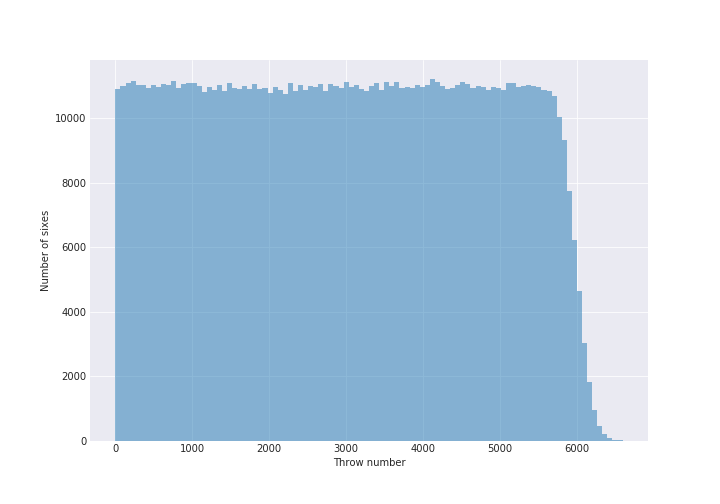

Simulations

Looks pretty good. The tail there is because we asked for 1000 sixes so some of the simulations took longer to get it. You could instead run the simulation for “t” seconds (or throws) and that would give you a nice looking boxy histogram.

Next, let’s see what the number of throws between sixes, or the wait times since we are throwing once per second, look like:

plt.figure(figsize=(10, 7))

wait_times = simulations[:, 1:] - simulations[:, :-1]
plt.hist(wait_times.ravel(), bins=20, alpha=0.5);
plt.annotate(text="Mean wait time: {:0.2f}".format(wait_times.mean()), xy=(0.11, 0.8),
             xytext=(0.15, 0.92), fontsize=14, xycoords='axes fraction', arrowprops= {'arrowstyle':"->"})
plt.axvline(x=wait_times.mean(), color='firebrick', ls="--")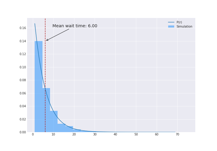

Simulations Wait Times

There’s the solution for (a). If you wanted to figure out what that distribution is, that’s easily enough. We know that probability that it take $r$ throws is the probability that we get something that is not a six for $r-1$ throws and then a six:

\[\mathbb{P}(r) = \left(\frac{5}{6}\right)^{r-1}\frac{1}{6}\]

The blue line in the figure above shows this function.

Clock strikes one

As per the exercise, let’s say that the clock strikes between two throws at some time $X$:

X = np.random.randint(0, high=simulations.max()//1.1)
X = X - 0.5

Note that $X$ is not really a random number (it happens at 1PM!) but to convince myself that this phenomenon is real, I ran this a number of times with different $X$s.

Let’s calculate the window around when the clock strikes:

def get_time_window(sim, X):

    before_strike = sim[sim < X]
    after_strike = sim[sim > X]

    if (len(after_strike) == 0) or (len(before_strike) == 0):
        return np.nan
    else:
        return after_strike.min() - before_strike.max()

window_around_strike = np.apply_along_axis(lambda a: get_time_window(a, X),
                                           1, simulations)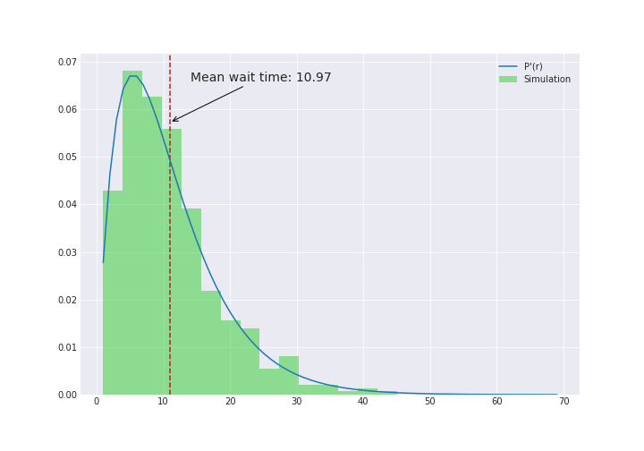

Simulations Wait Time Around Strike

Wow. Ok - so it is indeed 11 seconds instead of the 6 seconds.

So whats going on?

Here’s the CDF of the two windows above and we see that the window around the clock strike is indeed longer.

pdf_bias = np.histogram(window_around_strike, bins=40)[0]
cdf_bias = np.insert(np.cumsum(pdf_bias), 0, 0)
cdf_bias = cdf_bias / 1000

pdf = np.histogram(wait_times.ravel(), bins=40)[0]
cdf = np.insert(np.cumsum(pdf), 0 , 0)
cdf = cdf / cdf.max()
plt.figure(figsize=(10, 5))
plt.plot(cdf_bias, color='limegreen',
         label='CDF (# throws between 6s \naround clock strike)')
plt.axvline(window_around_strike.mean(), color='limegreen', ls = "--")
plt.plot(cdf, color='dodgerblue', label='CDF (# throws between 6s)')
plt.axvline(wait_times.mean(), color='dodgerblue', ls = "--")
plt.legend(loc=4, frameon=True)
sns.despine(left=True)
plt.grid(True, axis='both')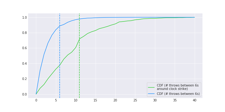

CDF

Let’s just look a small sample and see what’s going on. The figure below shows 10 simulations and 40 seconds before and after the clock strike. Each bar is a six being rolled. The red dotted line is when the clock strikes. The green area is the window from the six before the clock strikes and the blue area is the window to the next six after the clock strikes. Remember that the clock strikes between throws so we don’t need to worry about a six being thrown at the same time as when it strikes.

Sub-sample

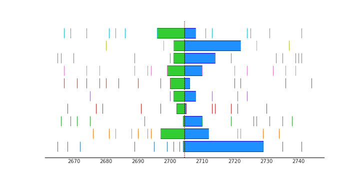
The mean window between sixes in just this sample shown is 5.9 and the mean of the window around the clock strike (green plus blue) is 11.9 rolls. We see that clock strikes seem to be in wide windows i.e. there is a large gap between sixes. So something similar to a the bus example is occuring.

The clock strike is more likely to occur between large gaps. It hurts my head to think about it this way since clock strike is predetermined (it strikes at 1). It’s not a random variable. But the way to think about it is that there are more events happening in large windows. Not just the clock striking but the dog barking, phone ringing, baby crying. There are just more seconds in those longer gaps for things to happen. So when looking from the perspective of some event occurring, it appears that the window is wider than average.

The probability of number of throws experienced around the event is not only related to the $P(r)$ but also to $r$; the longer the window between throws, the larger the probability that some event will happen within it. Let’s call the probability of the number of throws experienced around the event be $P’(r)$. The math is as follows (similar to the logic Jake VP has in his blog post):

\[\begin{aligned} \mathbb{P}'(r) &\propto r \mathbb{P}(r)\\ \mathbb{P}'(r) &= \frac{r \mathbb{P}(r)}{\int ^\infty_0 r \mathbb{P}(r) dr} \end{aligned}\]

The bottom is just $\mathbb{E}_{P}{[r]}$ and we know that to be six - the solution to part (a).

\[\begin{aligned} \mathbb{P}'(r) &= \frac{r \mathbb{P}(r)}{6}\\ \mathbb{P}'(r) &= r\left(\frac{5}{6}\right)^{r-1}\left(\frac{1}{6}\right)^2 \end{aligned}\]

This is the blue line in the figure in the previous section and we see that it matches our data quite well.

The bus analogy

If all this still makes you feel woozy (from the perspective of some unrelated event, the gaps between sixes is almost double) but the Poissonville bus analogy makes intuitive sense to you, hopefully drawing parallels between them will help:

Dice throwing

The dice is thrown every second
There are more seconds between longer spans without a 6
and therefore more likely that the clock strikes (or some event happens) between one of the longer spans.

Poissonville buses:

Passengers come every second (or uniformly)
There are more passengers waiting during longer spans without a bus
and therefore more likely that a passenger will be on a bus that was delayed

The notebook can be found here. You should also check out Jake VP and Allen Downey’s blogs mentioned above.

I need to get back to McKay’s book. So many more fun puzzles to solve!