This posts gives the Fader and Hardie (2005) model the full Bayesian treatment. You can check out the notebook here.
Here’s the first paragraph from the introduction introducing the problem:
Faced with a database containing information on the frequency and timing of transactions for a list of customers, it is natural to try to make forecasts about future purchasing. These projections often range from aggregate sales trajectories (e.g., for the next 52 weeks), to individual-level conditional expectations (i.e., the best guess about a particular customer’s future purchasing, given information about his past behavior). Many other related issues may arise from a customer-level database, but these are typical of the questions that a manager should initially try to address. This is particularly true for any firm with serious interest in tracking and managing “customer lifetime value” (CLV) on a systematic basis. There is a great deal of interest, among marketing practitioners and academics alike, in developing models to accomplish these tasks.
They construct a beta-geometric model to model the number of repeat transactions for a customer.
The model
All this is in the paper so I’ll go over it quickly. Here are the modeling assumptions:
-
If active, time between customer $i$’s transactions are a Poisson process:\
\[t_j - t_{j-1} \sim Poisson(\lambda_i)\] -
Each customer has her own $\lambda$ but it follows a gamma distribution\
\[\lambda \sim Gamma(\alpha, \beta)\] -
After (a key difference from the Pareto/NBD model) any transaction, customer $i$ can go inactive with probability $p_i$. So after
\[P(\text{i is in-active after j transactions}) = p_i(1 - p_i)^{j-1}\] -
Each customer has her own $p$ but it follows a beta distribution\
\[p \sim Beta(a, b)\]
Likelihood
F&H derive the following likelihood (eq. 3 in their paper):
\[L(\lambda, p | X=x, T) = (1 - p)^x\lambda^x e^{-\lambda T} + \delta_{x>0} p(1-p)^{x-1}\lambda_{x}e^{-\lambda t_x}\]If you try to implement this, you’ll quickly run into numerical issues. So let’s clean this up a bit:
\[\begin{aligned} L(\lambda, p | X=x, T) &= (1 - p)^x\lambda^x e^{-\lambda T} + \delta_{x>0} p(1-p)^{x-1}\lambda_{x}e^{-\lambda t_x}\\ L(\lambda, p | X=x, T) &= (1 - p)^x\lambda^x e^{-\lambda t_x} (e^{-\lambda(T - t_x)} + \delta_{x>0} \frac{p}{1-p})\\ \end{aligned}\]Taking logs to calculate the log-likelihood:
\[l(\lambda, p | X=x, T) = x log(1 - p) + x log(\lambda) - \lambda t_x + log(e^{-\lambda (T - t_x)} + \delta_{x>0}e^{log(\frac{p}{1-p})})\]Now that last term can be written using ‘logsumexp’ in theano to get around the numerical issues. Here’s an explanation for how it works. Numpy also has an implementation of this function.
PYMC3 model
You can get the data from here. I couldn’t find their test set online (for 39 - 78 weeks). Let me know if you find it.
Load the data
data_bgn = pd.read_excel("./bgnbd.xls", sheetname='Raw Data')

n_vals = len(data_bgn)
x = data_bgn['x'].values
t_x = data_bgn['t_x'].values
T = data_bgn['T'].values

int_vec = np.vectorize(int)
x_zero = int_vec(x > 0)       # to implement the delta function
Setup and run model
We need write our own custom density using the equation above. We’re working with tensors.
import pymc3 as pm
import numpy as np
import theano.tensor as tt

with pm.Model() as model:

    # Hypers for Gamma params
    a = pm.HalfCauchy('a',4)
    b = pm.HalfCauchy('b',4)

    # Hypers for Beta params
    alpha = pm.HalfCauchy('alpha',4)
    [id]: url "title" = pm.HalfCauchy('beta',4)

    lam = pm.Gamma('lam', alpha, r, shape=n_vals)
    p = pm.Beta('p', a, b, shape=n_vals)

    def logp(x, t_x, T, x_zero):

        log_termA = x * tt.log(1-p) + x * tt.log(lam) \
                                          - t_x * lam

        termB_1 = -lam * (T - t_x)
        termB_2 = tt.log(p) - tt.log(1-p)

        log_termB = pm.math.switch(x_zero,
                                  pm.math.logaddexp(termB_1, termB_2), termB_1)

        return tt.sum(log_termA) + tt.sum(log_termB)

        like = pm.DensityDist('like', logp,
                          observed = {'x':x, 't_x':t_x, 'T':T, 'x_zero':x_zero})
and let’s run it:
with model:
    trace = pm.sample(draws=6000, target_accept = 0.95, tune=3000)
Hyper-parameters
Remember that each customer $i$ has her own $p_i$ and $\lambda_i$. So let’s look at what the hyper-parameters look like:
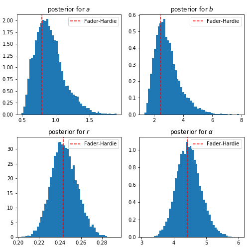
The mean value for each of these hyper-parameters is what Fader and Hardie get but we have the entire distribution.
Model Checks
You should do the Gelman-Rubin and Geweke tests at the least to make sure our model has converged. I won’t do it here but it’s in the notebook.
Posterior predictive checks
We can be pretty confident this model is right but it’s a good habit to do some posterior predictive checks so let’s do them anyway,
Usually we’d just run pm.sample_ppc and get some posterior predictives but that won’t work for us since we have a custom likelihood. Fader and Hardie derive $E(X(t)\vert\lambda,p)$ in equation 7. We can just use that formula to calculate the posterior predictives and see how well the models match the data observed.
p_post = trace['p']
lam_post = trace['lam']
expected_all = (1/p_post) * (-np.expm1(-lam_post * p_post * T))
Note that we factor out $\frac{1}{p}$ so allows us to use np.expm1 to avoid any overflow/underflow numerical issues. Theano and pymc3 also provide this function in case you need it while constructing a model.
Let’s see what this looks like. You can run this code multiple times to get a different random set of 16 customers and convince yourself that the model looks good:
# pick some random idx
idx = np.random.choice(np.arange(len(x)), size=16, replace=False)
f, axes = plt.subplots(4,4, figsize=(10,10))

for ax, i in zip(axes.ravel(), idx):
    _ = ax.hist(expected_all[:,i], density=True, alpha = 0.7, bins=20)
    _ = ax.axvline(x[i],ls='--', color='firebrick')
    _ = ax.set_title('cust: {numb}'.format(numb=i))
_ = plt.tight_layout()
This gives us the following plots.
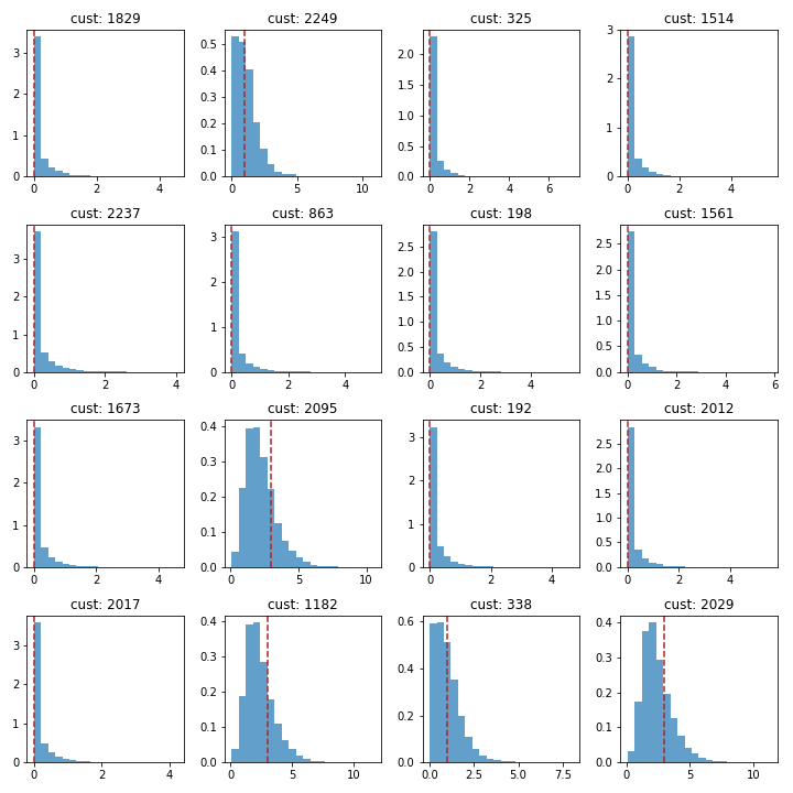
Looks pretty good to me though there seem to be some shrinkage for the large values. The data points (the line) are in the high probability region of the distribution of $E(X(t)\vert\lambda, p)$.
Why Bayesian
The mean values for $\alpha, r, a, b$ are around what Fader and Hardie find in their paper. So why do we bother setting up a full Bayesian model? The main advantage is that we now have a distribution so we can add some credible intervals when reporting the expected number of transactions for a customer. Also knowing the entire distribution, allows a business to design more effective targeting.
The cost is speed. Fader and Hardie use the optimizer in Excel to maximize the likelihood. In Python that would take you seconds and you have your pick of the latest optimizers. Running MCMC to draw samples from the posterior is slow. One option around it is to use variational inference to get approximations (check out the end of the notebook).
There are also other ways to get around this problem. You could use a “coreset”. Or you could assume hypers don’t change and just do a forward pass with new $x$ and $t_x$ and re-run the full model once every few months.