Empirical and Hierarchical Bayes

In chapter 2 of BDA3, the authors provide an example where they regularize the cancer rates in counties in the US using an empirical Bayesian model. In this post, I repeat the exercise using county level data on suicides using firearms and other means.

(maps won’t work if you have an ad-blocker. Disable it or allow this page for pretty maps: https://vega.github.io/vega-datasets/data/us-10m.json)

A lot of the methodology here is borrowed from BDA3. You should pick up that book if you want to check out the math at a deeper here. Unlike McElreath’s, you can’t easily read it cover to cover; it’s sometimes a little dense but I found it to be a good reference book. If you have the book (or check out the notebook), you’ll see that it has a 10 floating around. It’s so that we talk about 1 year death rates instead of the 10 years we have in the data. I’ve skipped that in the model specification below for clarity.

You can get the notebook here.

Data

I downloaded the data from CDC’s WONDER for the years 2007 - 2016 (inclusive). ICD-10 Codes X60 to X84 are for intentional self-harm and within that, codes X72, X73, and X73 relate to intentional self-harm using a firearm or handgun. I downloaded county population data from the US Census website since counties that have no suicides are not in the CDC WONDER dataset.

The problem

What is the suicide rate in each of the counties? We’ll model this first using empirical Bayes then repeat the exercise using hierarchical Bayes and note the differences between them.

The raw suicide rate

Since we have deaths by county, we can calculate the raw death rate as:

where $d_j$ is the number of deaths in county $j$ and the $pop_j$ is the population in county $j$.

Here’s what this looks like:

The next plot just highlights the counties with the highest and lowest rates:

Run your mouse over the counties and note that the both, lowest and highest rates, are in counties with small populations.

As Gelman et al point out in the kidney cancer example, though there may be a number of explanations for the difference in suicide rates, a large part of this variation can be explained by just one factor: sample size or, in our context, population size.

In a small county, with say a 50k people, if 1 person dies of suicide, the rate would be 1/50k = 0.00002 which would make it a pretty high suicide rate. If that one person does not die, it would be 0 and the lowest possible rate. Because the county has such a small population, one or two deaths can change the death rate drastically.

What we ideally want to do is ‘borrow’ some statistical power from the larger counties that have greater population sizes to regularize the death rate in the smaller counties. In other words, we want the posterior death rates to be dominated by an informative prior for noisy small-population counties and by the likelihood for large-population counties.

Why can we do this? Let’s say I tell you a county 997 has a suicide rate of 5 deaths per 100,000. This should influence what your estimate is for the suicide rate county 850. Especially if the sample size in county 997 was large. If you think that one county tells you nothing about another county then this model is flawed and we need to look at other ways of modeling it.

Coming up with a model

Let’s start by coming up with a generative model for these suicides. Let’s say that there is a $\theta_j$ that is the probability of a person committing suicide. So the likelihood $pi(d_j \vert \theta_j)$ is a Binomial:

Since we know $pop_j$ is large and $\theta_j$ is tiny, we can use the Poisson approximation for the Binomial:

Now we need a prior on $\theta$ that satisfies two constraints:

1. $\theta_j$ must be positive.
2. Most $\theta$s should be similar.

A gamma distribution satisfies both of these. Gamma is also the conjugate prior for a Poisson so it can be solved analytically. The posterior is just:

A beta distribution may also be nice and we also get the added benefit of constraining $\theta$ between 0 and 1 though that’s not that big of a deal. Coming up with the posterior and the prior predictive involves some algebra (and integrals) but that’s not a problem if we are using Monte Carlo methods.

Choosing prior parameters

Let’s choose a Gamma distribution as in BDA3. Now we need to choose appropriate $alpha$ and $beta$.

Empirical Bayes

We can use the data itself to come up with $\alpha$ and $\beta$. This is what puts the ‘empirical’ in empirical Bayes and is an approximation for the full bayesian treatment with hyper-parameters that we’ll do next.

The prior-predictive for our Poisson-Gamma model $d_i$ is Negative-Binomial.

Side note: Wikipedia has a very handy table with all the conjugate distributions.

The mean and variation of a Negative-Binomial are :

Let’s use the one sample that we have (starts sounding a little frequentist here), to match the moments, i.e. set the mean and variance of our sample to the moments and solve for $\alpha$ and $\beta$.

The following chart shows draws from $Gamma(\alpha, \beta)$ along with the distribution of $d_j$ or suicide rates from the data.

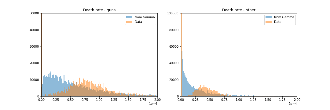
Not a great fit is it? It’s mainly because of that large mass at zero. If you squint, you may be able to convince yourself that the first two moments are indeed the same for the two distributions.

Running the models

We don’t really need to write any code here since we are working with conjugate pairs. But let’s do it anyway for fun.

with pm.Model() as mmatching:
    rate_gun = pm.Gamma('rate_gun', a_gun, b_gun, shape=len(suicides_gun))
    likelihood_gun = pm.Poisson('likelihood_gun', mu = 10*pop_gun*rate_gun,
                            observed = deaths_gun)

    rate_other = pm.Gamma('rate_other', a_other, b_other, shape=len(suicides_other))
    likelihood_deaths = pm.Poisson('likelihood_other', mu = 10*pop_other*rate_other,
                            observed = deaths_other)

The following plot shows the mean and hpd of the posterior of rate_gun.

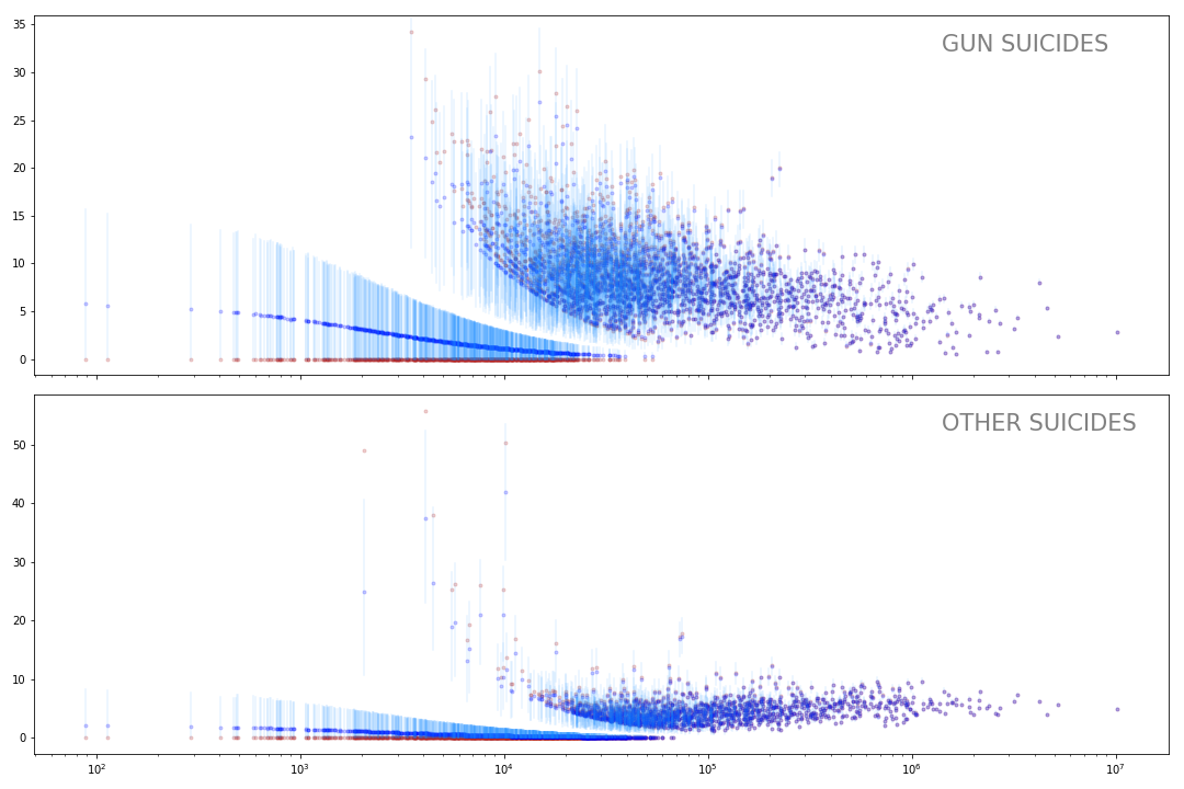
Note that the suicide rates for the small counties has been shrunk substantially and it has a pretty wide credible interval. That’s what you might expect. We can’t be confident on the exact suicide rate for the small counties but we know it’s probably higher than a zero.

Hierarchical Bayes

Instead of using the data to come up with values for the $\alpha$ and $\beta$ parameters of the Gamma prior, we could just create priors on these and let the model learn these.

So now our model is:

The first line is because $d_j$ is independent of $\alpha$ and $\beta$ when conditioning on $\theta_j$ i.e. $\alpha$ and $\beta$ effect $d_j$ only through $\theta_j$. The last line follows from $\alpha$ and $\beta$ being independent.

We need some priors on $\alpha$ and $\beta$. These hyper-parameters should be positive and can be large ($\beta from the empirical Bayes was around 400k), so let’s use a Half-Cauchy which has fat-tails allowing for large values.

Why 4? Because it seemed reasonable to me. You could choose a large number or call it a parameter $\tau$ and setup prior for that. Once you go high enough, and aren’t being too restrictive, it doesn’t make much of a difference.

Here’s the pymc3 code to run this model:

with pm.Model() as mhyper:
    alpha_gun = pm.HalfCauchy('alpha_gun', 4)
    beta_gun = pm.HalfCauchy('beta_gun', 4)

    alpha_other = pm.HalfCauchy('alpha_other', 4)
    beta_other = pm.HalfCauchy('beta_other', 4)

    rate_gun = pm.Gamma('rate_gun', alpha_gun, beta_gun, shape=len(suicides_gun))
    rate_other = pm.Gamma('rate_other', alpha_other, beta_other, shape=len(suicides_other))

    likelihood_gun = pm.Poisson('likelihood_gun', mu = 10 * rate_gun * pop_gun,
                            observed = deaths_gun)

    likelihood_other = pm.Poisson('likelihood_other', mu = 10 * rate_other * pop_other,
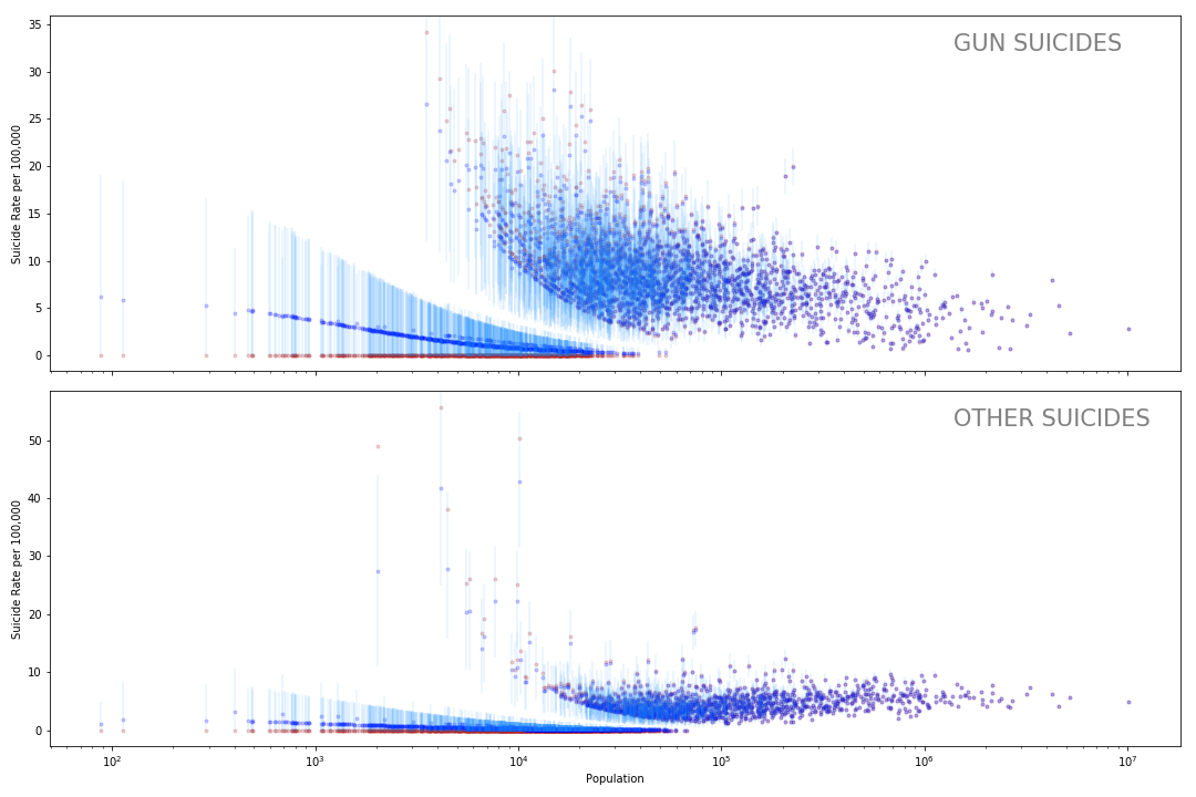
                            observed = deaths_other)

Here the plot again showing the mean and hpd of the posterior of rate_gun.

The plot below shows how the posteriors compare for the two models.

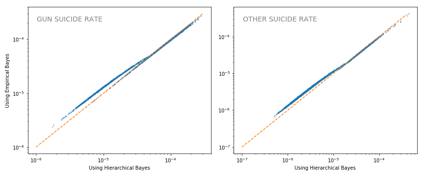
First, it’s remarkable how similar they are. At least in this context, empirical Bayes provides a decent approximation. Having said that, we see more shrinkage in the hierarchical model (more points above the orange 40 degree line).

Turtles all the way down

We are making an modeling assumption in the previous section: the parameters, $\theta$s, are exchangable. BDA3 describes it as follows:

“If no information – other that the data y – is available to distinguish any of the $\theta_j$s from any of the other, and no ordering or grouping of the parameters can be made, one must assume symmetry among the parameters in their prior distribution (page 104, ch5)”

This assumption might not really be true. We may believe that counties can be grouped by state or by how they voted in the last election. Say we want to do it by party. We can allow of different $\alpha$ and $\beta$ for each party and then tie them with another hierarchy. Here’s the pymc3 model:

with pm.Model() as mhyper_party:

    hyper_alpha = pm.HalfCauchy('hyper_alpha',1)
    hyper_beta = pm.HalfCauchy('hyper_beta',1)

    alpha_gun = pm.HalfCauchy('alpha_gun', hyper_alpha, shape=2)
    beta_gun = pm.HalfCauchy('beta_gun', hyper_beta, shape=2)

    alpha_other = pm.HalfCauchy('alpha_other', hyper_alpha, shape=2)
    beta_other = pm.HalfCauchy('beta_other', hyper_beta, shape=2)

    rate_gun = pm.Gamma('rate_gun', alpha_gun[party_gun], beta_gun[party_gun], shape=len(suicides_gun))
    #rate_other = pm.Gamma('rate_other', alpha_other[party_other], beta_other[party_other], shape=len(suicides_other))

    likelihood_gun = pm.Poisson('likelihood_gun', mu = 10 * rate_gun * pop_gun,
                            observed = deaths_gun)

    likelihood_other = pm.Poisson('likelihood_other', mu = 10 * rate_other * pop_other,

Since a lot of the red counties are tiny and the blue counties are huge coastal one, the shrinkage for the small counties is less:

Here’s a comparison of the shrinkage between the previous model and this ‘party’ model.

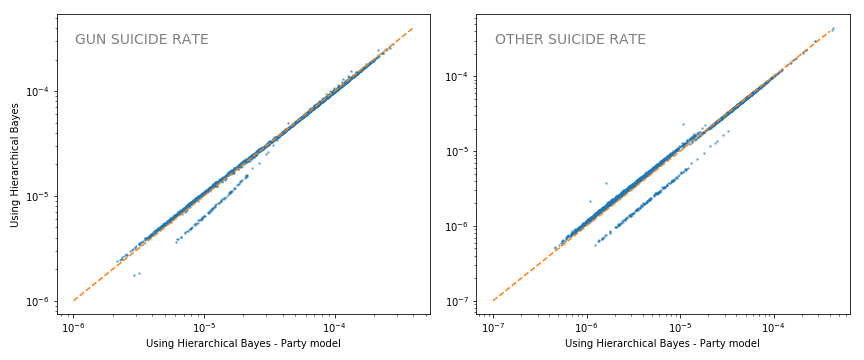
They are very similar except some counties (I’m guessing GOP ones) see less shrinkage.

What else?

Here are the two suicide rate posteriors means. We are only showing means but we have the whole distribution so really should keep the credible interval in mind. Some of the counties that seem to have very different rates may have significant overlap in their credible intervals.

This is a good starting point to do some deeper analysis.

It would be interesting to model the suicides in a county a little differently. Opponents of gun-laws often claim that people will find another way to commit suicide and having access to guns doesn’t really increase that rate.

We could setup a mixture model and see if this is indeed true. But may be for another time. These last two posts have been pretty morose and I need to model ice cream or puppies for a bit.