This is an implementation of SGDR based on this paper by Loshchilov and Hutter. Though the cosine annealing is built into PyTorch now which handles the learning rate (LR) decay, the restart schedule and with it the decay rate update is not (though PyTorch 0.4 came out yesterday and I haven’t played with it yet). The notebook that generates the figures in this can be found here.
Let’s talk about what SGDR is and then look at how it compares with step LR decay. Finally, we’ll look at how varying the two hyper-parameters, Ti and Tmult, affects performance.
SGDR intro
If you have done any sort of gradient descent type optimization, you’ll agree that tuning the learning rate is a pain. Techniques that use adaptive learning rates, like Adam, make life a little easier but some papers have suggested that they converge to a less optimal minima than SGD with momentum.
SGDR suggests that we use SGD with momentum with aggressive LR decay and have a ‘warm restart’ schedule. Here’s the formula from the paper for setting the LR, $\eta_t$, at run $t$:
\[\eta_t = \eta_{min}^i + \frac{1}{2}(\eta_{max}^i - \eta_{min}^i)(1 + \cos(\frac{T_{cur}}{T_i} \pi))\]Where:
- $\eta_{min}^i$ and $\eta_{max}^i$ are the minimum and maximum LR for the $i$-th run.
- $T_i$ is the number of epochs before we’ll do a restart.
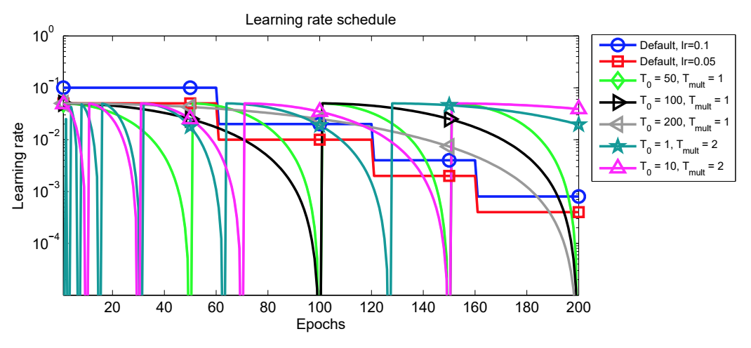
Another parameter that they mention is $T_{mul}$. They suggest increasing $T_i$ by a factor of $T_{mul}$ at each restart. Here’s the figure from the paper that shows the LR for for various values of $T_i$ and $T_{mul}$ and the step decay.
Authors show that using this method, you need fewer epochs to achieve a similar performance as some other learning rate schedules. Less epochs means less compute time.
The setup
We’ll just build off the standard tutorial for transfer learning in the pytorch docs. This is a model that uses resnet architecture and fine-tunes pre-trained weights to classify an image as an ant or a bee.
In the code in the notebook you’ll notice a few alterations from the model. We use a bigger model, resnet151, when comparing the SGDR and step decay. We also randomize the weights for 40 modules so that they need to be relearnt from the data. We do 20 runs and calculate the mean and standard deviation of the loss. We use seeds to ensure that the ‘randomness’ in SGD (what’s in a batch etc.) is the same for the models.
We are only using a small number of images to make it fast but you should try it for bigger datasets (there is a furniture classification competition on kaggle right now).
SGDR vs. step decay
Note that I use a step-size of 60 and a gamma of 0.1 in the step decay LR model. This is coming straight from the tutorial. You may want to play with this and see what gamma and step-size give the lowest loss under this scheme. We also use 10 and 2 for Ti and Tmult respectively. These are values that the authors find works well for them.
Here’s what the loss looks like. The shaded areas shows the 1 standard deviation bounds.
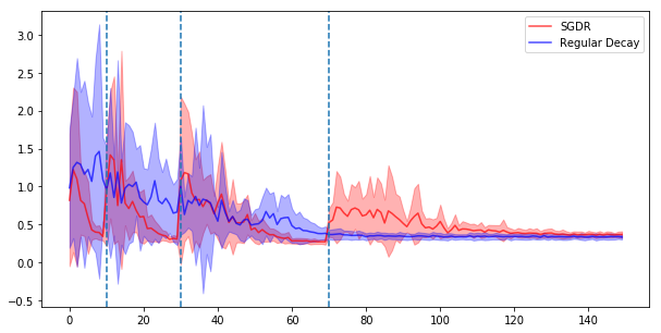
The authors note that we should be looking at the loss at the end of a cycle since it’s going to be bouncing all over the place early on when the LR is high. Looks like we get to a minimum pretty quickly. After just 10 epochs we seem to have hit a minimum. It jumps back out and find another minima after 30 epochs again. Meanwhile, step decay gradually improves it’s performance and seems to real a minima around the 65th epoch.
Effect of tuning hyper-parameters
We re-ran SGDR with resnet50 with the parameters for Ti and Tmult suggested in the paper. Here’s what it looks like.
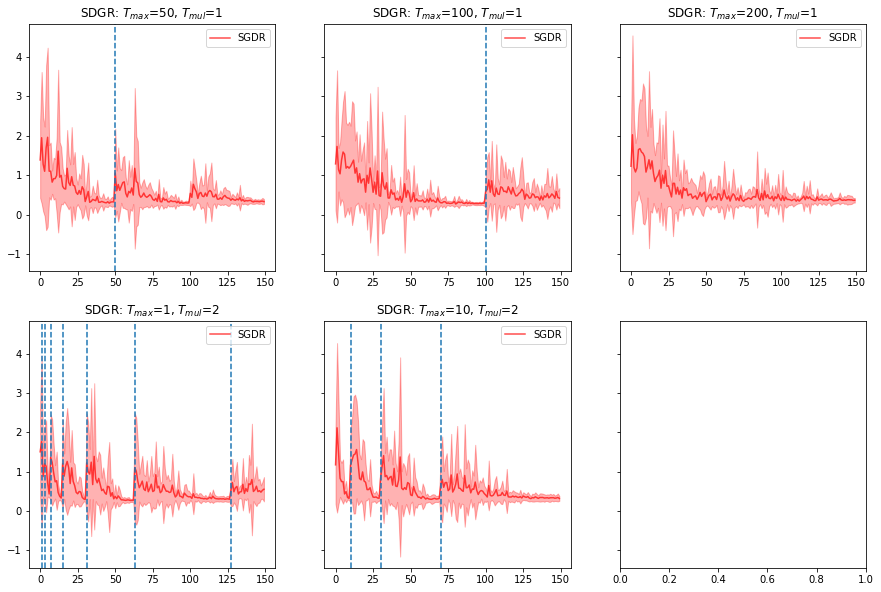
Bit hard to compare them but it shows the standard deviation which is useful to know how consistent it is at finding the minima.
Let’s compare the mean performance for these (with some RBF smoothing):
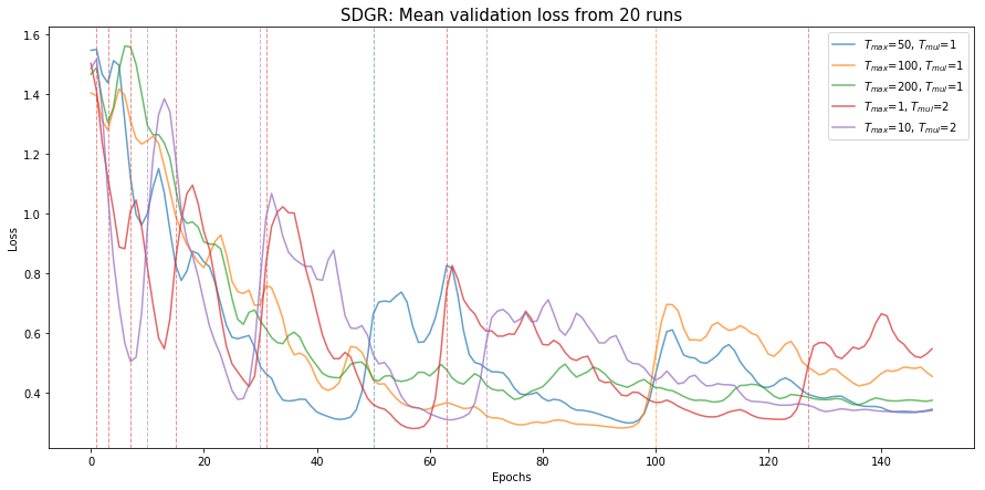
Ti and Tmult values of 1 and 2 respectively seems to be the best for our problem; the minima reached on the 59th epoch by these models is the lowest. Going back to the previous figure, we also note that the variation around this is tiny so we have some measure of confidence that these are indeed the hyper-parameters we should go with.
Want to play some more?
Though this specific paper implements this on a SGD with momentum optimizer, the same authors showed that you can do it with Adam as well. Give it a go.
The advantage of SGDR is that you need fewer epochs to reach the minima. And the minima found at the end of each cycle may be a different one. They show that taking an ensemble of models at these different minima can improve predictive performance. We don’t do this here but it’s easy enough to save weights at the end of each cycle (the code for keeping the best model is up, it just needs to be tweaked to keep a set of them).
Other references
You should check out the paper. There is a lot more in it and I gloss over a few details here. Sebastian Ruder had a nice blog post that summarizes a number of recent advances in improving optimization in deep learning.
Distill had an amazing blogpost (the kind only a team like that could produce) that explains a lot of these method with some nice visualizations.