If you didn’t see Part 1, check that out first.
I did promise an actual example. Here’s an example of using SA for a simple Nurse Scheduling Problem.
I want to talk a little bit more about this line:
alpha = min(1, e^((E_old - E_new)/T) # (3)Let’s explore what exactly is going on here. Say we have a function f(x) as follows:
\[f(x) = -5(x)^2 + \frac{1}{6} \cdot x^3 + \frac{1}{2} \cdot x^4 + 20\]Let’s see what this looks like:
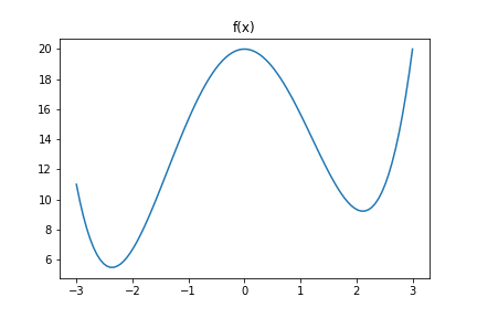
So we have a local minimum and a global minimum. Now let’s see what the values of alpha is as we change T (I have removed alpha = 1 for clarity). I have generated a bunch of random points for $x_{old}$ and $x_{new}$ between -3 and 3.
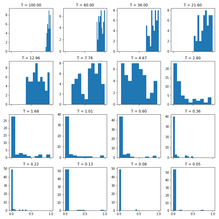
Alpha is closer to 1 when temperature is high and is closer to 0 when temperature is low. Alpha comes into play here:
if (E_new < E_old) or (alpha > threshold):where threshold was drawn from a uniform distribution. In terms of our example, if $f\left(x_{new}\right)$ is less than $f\left(x_{old}\right)$ then accept. If not, check if alpha is greater than the random draw. If temperature is high and we’re getting alphas around 0.9, they’ll be accepted around 90% of the time. If temperature is low and we’re getting alphas around 0, then almost none will get accepted.
So when temperature is high, we accept an x even if f(x) is higher than our current estimate. The importance of the proposal function being able to ‘communicate’ between any two points is clear now. If not, we’ll never propose an x way out there, and we’ll never explore that part of the space. We’ll be stuck around our current minima.
Finally, what exactly does $e^{f(x)/T}$ look like?
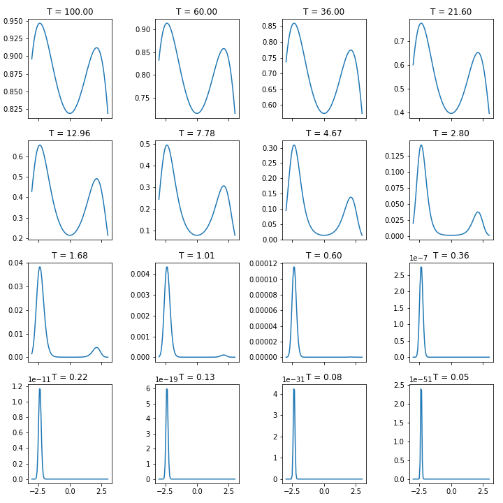
Note that the y-axes have different scales. When temperature is high, the difference between being in different regions is not that great. Which means that $\frac{e^{f(x_{old})/T}}{e^{f(x_{new})/T}}$ is around 1. Later on, it resembles a delta function where unless you are proposing something very very close to global minimum, you’re getting an alpha of pretty much 0 which means you’re now just fine tuning around the minimum.
Actually, what we are doing is drawing from a different Boltzmann distribution at each T:
\[\displaystyle p_{i}={\frac {e^{-{\varepsilon }_{i}/kT}}{\displaystyle \sum _{j=1}^{M}{e^{-{\varepsilon }_{j}/kT}}}}\]Note that the denominator term just normalizes the distribution and we use k=1.
Wait, we are drawing from a distribution? So can we draw from any other distribution? That leads us nicely to sampling using Metropolis. You can head on to Part 3 or if you need a little motivation, check out this post on Monte Carlo methods and this one on Why MCMC (and intro to Markov Chains).
If you want to run this yourself, you can get the notebook from here.